CHE 318 Lecture 02
Molecular Diffusion in Gases: Diffusive + Convective Mass Transport
2026-01-07
Recap
Fick’s 1st law of diffusion \[ J_{Az}^{*} = -D_{AB}\dfrac{d c_A}{dz} \]
Diffusion and convection \[ N_{A} = J_{Az}^{*} + c_A v_m \]
Governing equation for binary mixture system \[ N_{A} = -c_T D_{AB} \dfrac{d x_A}{dz} + x_A(N_A + N_B) \]
We will learn how to solve this equation in this lecture!
Learning outcomes
After this lecture, you will be able to:
- Recall the difference between diffusion and convection mechanisms in binary mixtures.
- Identify common transport cases from the relation between \(N_A\) and \(N_B\).
- Describe the governing constraint for a given gas-diffusion setup.
- Apply flux equations for equimolar counter diffusion and diffusion through stagnant B.
- Analyze how the stagnant-B assumption changes concentration profiles and driving forces.
Recap: Fick’s 1st law of diffusion
Diffusion flux of A in B, z-direction follows:
\[ J^*_{Az} = - D_{AB}\,\frac{d c_A}{d z} \]
- Fick was the first to propose the relation between diffusion and concentration gradient driving force
- Analog:
- Heat transfer (Fourier’s law)
- Momentum transfer in fluid (Newton equation)
- Diffusivity \(D_{AB}\) was later linked to molecular Brownian motion by Albert Einstein
- \(D_{AB}\) has unit of \(\mathrm{m^2\,s^{-1}}\)
Behaviour of molecular diffusion
- Brownian motion (Bm) is the inherent motion of molecules
- Bm leads to redistribution of molecules until \(\dfrac{d c_A}{d z} = 0\)
- Non-zero flux only when \(\dfrac{d c_A}{d z} \neq 0\)
- Is diffusivity temperature dependent? pressure dependent?
- How fast is molecular diffusion?
Typical \(D_{AB}\) range
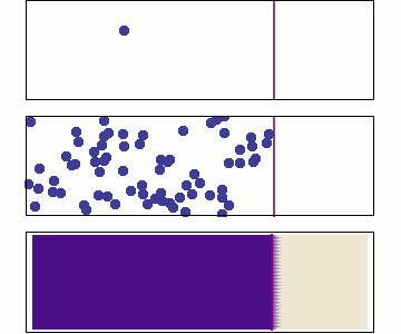
A common misconception
Search for any youtube video with “diffusion experiment dye”
Can we verify whether the scenario seen is Fickian diffusion?
Diffusion vs convection length scale
Length \(L\) traveled in time \(t\):
- Diffusion: \(L = 6\sqrt{D_{AB}\,t}\) (Einstein, ~1905)
- Convection: \(L = v_m\,t\)
What is typical \(D_{AB}\) in a liquid?
- Often \(D_{AB}\sim 10^{-9}\) to \(10^{-10}\,\mathrm{m^2/s}\)
Assuming \(D_{AB} = 10^{-10} \mathrm{m^2/s}\) \(v_{m} = 10^{-3} \mathrm{m/s}\)
Diffusion vs convection summary
Diffusion
- Driven by concentration gradient
- Associated with Diffusivity \(D_{AB}\)
- Diffusive velocity \(v_{Ad}\)
- Slow at large (industry) length scale
Convection
- Driven by bulk motion
- Can reinforce or oppose diffusion
- Bulk fluid motion \(v_m\)
- Fast at large (industry) length scale
A note on setups
Reference frame
- \(J_{Az}^{*}\) refers to the fluid plane frame (hence the \(*\))
- \(N_{A}\) refers to the stationary frame (lab frame)
- We will be dealing with \(N_A\) in this course!
Mass balance in stationary frame
\[ [\mathrm{In}] - [\mathrm{Out}] + [\mathrm{Generate}] = [\mathrm{Accumulation}] \]
Steady state (S.S)
- \([\mathrm{Generate}] = [\mathrm{Accumulation}] = 0\)
- \([\mathrm{In}] = [\mathrm{Out}]\)
- \(\dfrac{d N_A}{dz} = 0\) (S.S)
Governing equation for \(N_A\) and \(N_B\)
The common way of expressing the governing equation is
\[\begin{align} N_{A} &= -c_T D_{AB} \dfrac{d x_A}{dz} + x_A(N_A + N_B) \\ N_{B} &= -c_T D_{BA} \dfrac{d x_B}{dz} + x_B(N_A + N_B) \end{align}\]How can we solve these?
- For this course we assume \(D_{AB}\) and \(D_{BA}\) are constants
- For industrial purposes we want to know values of \(N_A\) and \(N_B\)
- We need relation between \(N_A\) and \(N_B\) to solve them!
- \(x_A(z)\) can be solved as a by-product
Three limiting cases
Equimolar Counter Diffusion (EMCD)
Assumption
- \(N_A + N_B = 0\)
- \(v_m = 0\)
Example
- Two gases exchanging through a thin tube
- Idealized membrane diffusion
Diffusion with Stagnant B
Assumption
- \(N_B = 0\)
- \(N_A \neq 0\)
Example
- Evaporation of A through non-diffusing air
- Gas absorption into a liquid film
General Case
Assumption
- \(N_A \neq 0\)
- \(N_A = k N_B\) (\(k \neq -1\))
Example
- Catalyst reaction
Case 1: equimolar counter diffusion (EMCD)
- Condition: \(N_A + N_B = 0\)
- No bulk fluid motion
Relation in EMCD gives:
\[\begin{align} c_T D_{BA} \dfrac{d x_B}{d z} &= -c_T D_{AB} \dfrac{d x_A}{d z} \end{align}\]Since \(x_A + x_B = 1\), we have \(D_{AB} = D_{BA}\)
Solving EMCD: flux \(N_A\)
Assume S.S., constant \(D_{AB}\) and integrate from \(z_1\) to \(z_2\)
\[\begin{align} \int_{c_{A1}}^{c_{A2}} d c_A &= -\frac{N_A}{D_{AB}} \int_{z_1}^{z_2} d z \\ c_{A2} - c_{A1} &= -\frac{N_A}{D_{AB}}(z_2 - z_1) \\ \end{align}\] \[\begin{align} \boxed{ N_A = \frac{D_{AB}}{(z_2 - z_1)}(c_{A1} - c_{A2}) } \end{align}\]For ideal gas:
\[\begin{align} \boxed{ N_A = \frac{D_{AB}}{RT(z_2 - z_1)}(p_{A1} - p_{A2}) } \end{align}\]Case 2: diffusion through stagnant B
Definition: stagnant species B means zero molar flux in the lab frame: \[ N_B = 0 \]
But diffusion in B phase still occurs!
The governing equation becomes:
\[\begin{align} N_A &= -c_TD_{AB}\dfrac{d x_A}{dz} + x_A N_A \\ N_A(1 - x_A) &= -c_TD_{AB}\dfrac{d x_A}{dz} \end{align}\]Solving stagnant B case
We again do an integration by separating variables:
\[\begin{align} \frac{d x_A}{1-x_A} &= -\frac{N_A}{c_TD_{AB}}\,dz \\ \int_{x_{A1}}^{x_{A2}} \frac{d x_A}{1-x_A} &= -\frac{N_A}{c_TD_{AB}}\int_{z_1}^{z_2} dz \\ \left[-\ln(1-x_A)\right]_{x_{A1}}^{x_{A2}} &= -\frac{N_A}{c_TD_{AB}}(z_2-z_1) \\ \ln\!\left(\frac{1-x_{A1}}{1-x_{A2}}\right) &= -\frac{N_A}{c_TD_{AB}}(z_2-z_1) \end{align}\] \[\begin{align} \boxed{ N_A = \frac{c_TD_{AB}}{(z_2-z_1)} \ln\!\left(\frac{1-x_{A2}}{1-x_{A1}}\right) } \end{align}\]Various forms of stagnant B solution
- In concentration and molar fraction
- Ideal gas with partial pressure
Log-mean form
Historically, engineers liked to write the stagnant B equation using linear terms.
\[\begin{align} \ln\!\left(\frac{p_T-p_{A2}}{p_T-p_{A1}}\right) &= \ln\!\left(\frac{p_{B2}}{p_{B1}}\right) \\ (p_{B2} - p_{B1})\ln\!\left(\frac{p_T-p_{A2}}{p_T-p_{A1}}\right) &= \ln\!\left(\frac{p_{B2}}{p_{B1}}\right) (p_{A1} - p_{A2}) \\ \ln\!\left(\frac{p_T-p_{A2}}{p_T-p_{A1}}\right) &= \ln\!\left(\frac{p_{B2}}{p_{B1}}\right) \left( \frac{p_{A1} - p_{A2}}{p_{B2} - p_{B1}} \right) \end{align}\]Define \(p_{Bm} = \dfrac{p_{B2} - p_{B1}}{\ln\!(p_{B2}/p_{B1})}\)
We get
\[\begin{align} N_A = \frac{D_{AB}}{RT(z_2-z_1)} \frac{p_T}{p_{Bm}}(p_{A1}-p_{A2}) \end{align}\]Solving concentration profiles in stagnant B
- We will utilize the fact \(d N_A / dz = 0\) (S.S).
- Do we have \(d c_A / dz = 0\) like in EMCD?
Can you solve the profile for \(x_A(z)\)?
Summary
- Choosing the right transport constraint is the key first step in solving binary diffusion problems.
- Equimolar counter diffusion leads to linear concentration and partial-pressure profiles.
- Diffusion through stagnant B produces non-linear profiles and a logarithmic driving-force form.
- The statement “stagnant B” means \(N_B = 0\), not “no diffusion.”
Next lecture: we remove simplifying constraints and discuss the general case