CHE 318 Lecture 21
In-Depth Analysis of Packed Bed Columns
2026-03-02
Learning outcomes
After this lecture, you will be able to:
- Recall how packed-bed mass transfer coefficients compare with those of other geometries.
- Describe mass-balance equations for packed-bed columns.
- Identify concentration and pressure profiles inside a packed column.
Recall from last week: mass transfer correlations
Goal: calculate \(k_c'\) from:
- geometry (\(L_D, L, D_P\), etc)
- properties (\(\mu, \rho, D_{AB}, v\), etc)
Calculate \(N_{\text{Re}}\), \(N_{\text{Sc}}\)
Get \(j_D\) and / or \(N_{\text{Sh}}\) to back-calculate \(k_c'\)
A deeper look into packed bed

Recall from last week: comparison between geometries
Adapted from Problem 7.3-3. Let’s estimate the gas-phase mass transfer coefficient \(k_G\) (kg mol/(m\(^2\) s Pa)) for mass transfer of water vapour to solids with different shapes. Consider a water vapour (A) in air (B) at 338.6 K and 101.32 Pa flowing through a big duct containing solids with various geometries. The flow velocity is 3.66 m/s. The water vapour concentration is small, so property of air is used (\(\mu=2.03\times 10^-5\) Pa\(\cdot\)s, \(\rho=1.043\) kg/m\(^3\)). From the table, \(D_{AB} = 2.88 \times 10^{-5}\) m\(^2\)/s at 315 K. Compare the values for following geometries, which case?
- Flow parallel to flat plate with length \(L=2.54\) cm
- A single sphere with diameter \(D=2.54\) cm
- Packed beds using spheres of average diameter \(D_p=2.54\) cm and \(\epsilon=0.35\)
Case 3: results
Tip
- Do not forget to correct \(D_{AB}\) for temperature!
- Choose the right \(N_{\text{Sh}}\) or \(j_D\) formula according to \(N_{\text{Re}}\) and \(N_{\text{Sc}}\)
- \(k_G \approx k_G' = k_c' / (RT)\)
- Flat surface: \(k_G = 1.738\times 10^{-8}\) kg mol/(m\(^2\) s Pa). \(N_{\text{Sh}} = 38.03\)
- Single sphere: \(k_G = 1.984\times 10^{-8}\) kg mol/(m\(^2\) s Pa). \(N_{\text{Sh}} = 43.40\)
- Packed bed: \(k_G = 7.60\times 10^{-8}\) kg mol/(m\(^2\) s Pa). \(N_{\text{Sh}} = 166.32\)
Packed bed clearly wins!
Why packed bed columns have better mass transfer?
Packed bed geometry provides large surface-to-volume ratio (\(\epsilon\) and \(D_p\))
The boundary layer length \(\delta c\) is small due to continuous disruption of liquid/gas interface
Overall \(k_c'\) is larger than single geometry
Pressure drop \(\Delta p\) over the column can be larger than other types!
Compute mass transfer in packed bed columns
In a packed bed design, it is often desired to know the following quantities:
- The outlet concentration \(c_{A2}\)
- The total flux of mass transfer across interface
- It is still desired to use [In] - [Out] + [Gen] = [Acc]
- What are each of these quantities?
Mass balance in packed beds
- Volumetric flow rate is \(Q\) (unit m\(^3\)/s)
- Inlet, outlet concentration: \(c_{A1}\), \(c_{A2}\)
- Cross sectional area \(S\)
- Interfacial mass transfer flux \(N_A\), effective area \(A_{\text{eff}}\)
The effective area \(A_{\text{eff}}\)
- \(A_{\text{eff}}\) related to the surface-to-volume ratio \(a\) and total bed volume \(V_b\)
- For spheres, we can derive \(a\) (unit m\(^2\)/m\(^3\))
How to get \(\hat{N}_A\)?
- \(\hat{N}_A\) is the average mass transfer flux across the interface.
- To solve it, we still use a control volume from \(z\) to \(z+ dz\)
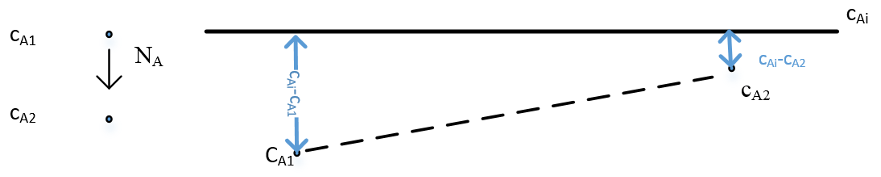
- Locally, driving force \(c_{Ai} - c_{A}(z)\)
- Local mass transfer flux
Differential equation for \(c_A(z)\)
\[\begin{align} N_A a S dz &= Q d c_A \\ \frac{k_c a S}{Q} dz &= \frac{d c_A}{c_{Ai} - c_{A}(z)} \end{align}\]Integrating over \(z\) we get:
\[\begin{align} \ln\!\left( \frac{c_{Ai} - c_{A1}}{c_{Ai} - c_{A}(z)} \right) = \frac{k_c a S z}{Q} \end{align}\]Concentration profile of packed bed (single phase)
- When \(c_{Ai}\) is constant (e.g. solid-gas interface), concentration follows:
- Analog: reactive wall in pipe system (unsteady-state mass transfer in Lecture 11)
The pipe wall problem corresponds to \(a=4 / D\), similar to a packed bed problem.
- Clearly, packed bed can achieve saturation much faster, because \(D_p\) is usually a few mm to 1 inch.
Outlet concentration for packed bed
- If a packed bed column has height \(H\), outlet concentration \(c_{A2}\) follows:
- Rearrange gives
Solving the average mass transfer flux \(\hat{N}_A\)
- We can further use the mass balance equation \(Q(c_{A1} - c_{A2}) + \hat{N}_A A_{\text{eff}} = 0\).
- Use the fact \(c_{A2} - c_{A1} = (c_{Ai} - c_{A1}) - (c_{Ai} - c_{A2})\)
That gives us
\[ \hat{N}_{A} = k_c \frac{(c_{Ai} - c_{A1}) - (c_{Ai} - c_{A2})}{\ln\!\left( \frac{c_{Ai} - c_{A1}}{c_{Ai} - c_{A2}} \right)} \]
Average mass transfer flux by log-mean driving force
The previous result means the average driving force in a exponentially-changing concentration profile like in packed bed, should be expressed in log-mean driving force form.
It is an expression we will frequently see in other column setups with mixing interfaces
\[ \hat{N}_{A} = k_c \frac{(c_{Ai} - c_{A1}) - (c_{Ai} - c_{A2})}{\ln\!\left( \frac{c_{Ai} - c_{A1}}{c_{Ai} - c_{A2}} \right)} \]
Example 4: packed bed design
In this lecture, we show that the outlet concentration will be saturated when the tube is long enough.
\[\begin{align} c_{A2} = c_{Ai} - (c_{Ai} - c_{A1})\exp(- \frac{A k_c}{Q}) \end{align}\]- Consider all parameters in case 3, how high should we design the packed bed to ensure saturated outlet concentration?
- \(D_p=2.54\) cm, \(\epsilon=0.35\), \(k_c'=0.214\) m/s, \(v_m=3.66\) m/s
- You can consider effective saturation means \(\frac{A k_c}{Q} = 5\)
Example 4: packed bed design – results
- Minimal height: \(H_{\text{min}}\)
\[ H_{\text{min}} = \frac{5 v_m D_p}{6 (1 - \epsilon) k_c'} \]
- In case 3 setup, \(H_{\text{min}}=0.556\) m
Summary
- Dimensionless numbers can be used to correlate mass transfer problems in different flow rate, dimension etc
- Typically, start with a known geometry (pipe? parallel plate? sphere? packed bed?)
- Find the correlation with dimensionless numbers \(N_{Re}\), \(N_{Sc}\)
- Calculate the final mass transfer rate