MATE 664 Lecture 02
Introduction to Irreversible Thermodynaics
2026-01-07
Recap of Lecture 01 (Big Picture)
Key ideas from last lecture:
- Thermodynamics tells us whether a process can occur
- Kinetics tells us how fast it occurs
- Equilibrium depends on time scales, not perfection
- Free energy change \(\Delta G^{0}\) determines spontaneity
- Activation barrier \(\Delta G^*\) controls rates
Recap: equilibrium is a time-scale concept
- Equilibrium when
\[\tau_{\text{observation}} \gg \tau_{\text{relaxation}}\]
- Many materials are metastable, not unstable
- Diamond vs graphite is a kinetic story, not thermodynamic failure
Recap: entropy revisited
- Entropy is not disorder
- Entropy measures number of accessible microstates
- Statistical view:
\[S = k_B \ln\!\Omega\]
Learning outcomes
After this lecture, you will be able to:
- Describe why classical thermodynamics is insufficient for real kinetic processes
- Define entropy production and irreversible processes
- Relate macroscopic fluxes to thermodynamic driving forces
- Apply Onsager’s linear response framework
- Interpret irreversible thermodynamics from a microscopic viewpoint
Crash course on statistical mechanics (1)
Part of the introductions are adapted from MAT E 374 by Dr. Hao Zhang
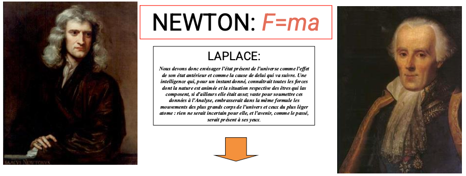
Dynamics from Newton & Laplace point of view:
- Transition from state A to B is deterministic
- We just need to know \(\{\mathbf{x}_i, \mathbf{v}_i, F_{ij}\}\)
Newtonian dynamics in a nutshell
Crash course on statistical mechanics (2)
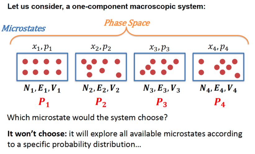
Why can’t we determine the system state using Newtonian Dynamics (yet)?
- Astronomical numbers of microstates
- Limitation of computational power
- Waste of computational power
What is the alternative?
- Deterministic -> probabilistic
- How much computation is enough?

Crash course on statistical mechanics (3)
Let’s reintroduce the microscopic picture by Boltzmann
Crash course on statistical mechanics (4)
- Microstate: a state in the phase space \(\{\mathbf{x}_i, \mathbf{p}_i\}\)
- Macrostate: a specification of macroscopic constraints (e.g. \(<E, V, N>\)) that corresponds to many microstates
- Ensemble: a set of constraints like \(<E, V, N>\) describing the system
Central principle linking macrostate and microstates:
The observed macroscopic thermodynamic property \(A_{obs}\) is an ensemble average of all possible microstates \(i\)
\[ A_{obs} = \langle A \rangle = \sum_i A_i \, p_i \]
Crash course on statistical mechanics (5)
Consider a canonical ensemble (constant \(N, V, U\)) 1
- Inner system (I): \(U_I\), \(\Omega(U_I)\)
- Reservoir system (R): \(U_R\), \(\Omega(U_R)\)
- Total system (universe, T): \(U_T = U_I + U_R\), \(\Omega(U_T) = \Omega(U_I) \times \Omega(U_R)\)
- \(U_R \gg U_I\)
I and R can only exchange internal energy, not particles or volume.
Q: The total internal energy of the universe \(U_T\) is fixed. How do the inner and reservoir systems balance their energies?
Crash course on statistical mechanics (6)
Let’s first see the equilibrium state.
- Assume at e.q., we have \(U_I = U_I^{0}\)
- Probability of inner energy follows how many states in the reservoir they can exchange with:
\[P(U_I) \propto \Omega(U_T - U_I^0)\]
- Since \(U_T \approx U_R \gg U_I^0\), we can use Taylor series for \(\Omega(U_T - U_I^0)\):
\[ \ln\!\Omega(U_T - U_I^0) = \ln\!\Omega(U_T) - \frac{\partial \ln\!\Omega}{\partial U} \bigg\vert_{U=U_T} \cdot U_I^0 + \dots \]
Crash course on statistical mechanics (7)
- We know the Boltzmann equation \(S = k_B \ln\!\Omega\)
\[ \ln P(U_I^0) \propto \ln\!\Omega(U_T) - \frac{\partial S_T}{k_B \partial U} \bigg\vert_{U=U_T} \cdot U_I^0 \]
Recall the classical thermodynamic relation:
\[ dU = TdS - pdV \]
We have \(\dfrac{\partial S}{\partial U}\bigg\vert_{V} = \dfrac{1}{T}\), therefore
\[ P(U_I^0) \propto \Omega(U_T) \exp(-\dfrac{U_I^0}{k_B T}) \]
This leads the famous Boltzmann distribution
Crash course on statistical mechanics (8)
What if we’re not at equilibrium?
\(T_I\) and \(T_R\) may be two distinct values.
We will apply local equilibrium assumption here
One postulate for stat. mech. is that the entropy of the universe always increases.
We go further by say the equilibrium maximizes the universe entropy
\[ \left( \dfrac{ \partial \ln \Omega(U_T) }{\partial U_I} \right)_{N, V, U} = 0 \]
- Can we make sure it is the maximum?
- What is the sign of \(\partial^2 S/\partial U^2\)?
Crash course on statistical mechanics (9)
\[ \left( \dfrac{ \partial \ln \Omega(U_I) }{\partial U_I} \right)_{N, V, U} + \left( \dfrac{ \partial \ln \Omega(U_R) }{\partial U_I} \right)_{N, V, U} = 0 \]
Use the relation \(\partial U_I = -\partial U_R\)
\[ \left( \dfrac{ \partial \ln \Omega(U_I) }{\partial U_I} \right)_{N, V, U} = \left( \dfrac{ \partial \ln \Omega(U_R) }{\partial U_R} \right)_{N, V, U} \]
Apply Boltzmann equation
\[ T_I^{-1} = T_R^{-1} \]
Yay! This is something we know, temperature at equilibrium.
What have we observed so far?
- Probability distribution at equilibrium follows Boltzmann distribution (for canonical ensemble)
- Equilibrium is a consequence of maximizing entropy of the universe
- We can locally apply the equilibrium thermodynamics to describe kinetic process (though we don’t know how fast yet)
Formal framework
In Onsager’s Irreversible Thermodynamics, for any thermodynamic parameter \(X\), we define
Affinity \(F\): the influence of \(X_i\) to the universe entropy \[ F_i = \frac{\partial S}{\partial X_i} \]
Flux \(J\): the change of parameter \(X_i\) (or density of it) per unit time \[ J_i = \frac{d X_i}{d t} \]
Kinetic Coefficient \(L_{ij}\): influence of flux type \(i\) by affinity type \(j\) (linear term). \[ L_{ij} = \dfrac{\partial J_i}{\partial F_j} \]
Postulate 1: local equilibrium
It is generally possible to use principles of the continuum limit to define meaningful, useful, local values of various thermodynamics quantities, e.g., chemical potential \(\mu_i\).
Useful kinetic theories can be developed by assuming a functional relationship between the rate of a process and the local departure from equilibrium (“driving force”).
Postulate 2: entropy production
Irreversible Process is An Increase of Entropy in the Universe
\[ \frac{dS}{dt} = \sum_i \frac{\partial S}{\partial X_i} \frac{\partial X_i}{\partial t} = \sum_i F_i J_i \]
- Entropy can be created in the universe
- Entropy can flow between micro-systems
- Rate of entropy production (entropy generation + flow) must be positive
Postulate 3: linearity
- The relation between \(J\) and \(X\) can be linearly described (resistive system).
- Flux is only dependent on the affinity at the same time
Or in vector term \[ \mathbf{J} = \mathbf{L}\cdot\mathbf{F} \]
- Coefficient \(L_{ii}\) is called direct kinetic coefficient
- Affinity \(F_{i}\) is called conjugate driving force w.r.t. \(J_i\)
- Coefficient \(L_{ij}(i\neq j)\) is called coupling coefficient
Postulate 4: reciprocity
Onsager proposed that
\[ L_{ij} = L_{ji} \]
This is a key component in material kinetics!
Summary
- Irreversible processes are driven by thermodynamic forces
- Each force generates a corresponding flux
- Near equilibrium, fluxes depend linearly on forces
- Empirical transport laws (Fourier, Ohm, Fick) are special cases of: \[ J_i = \sum_j L_{ij} F_j \]
- Onsager reciprocity enforces symmetry: \[ L_{ij} = L_{ji} \]