MATE 664 Lecture 03
Driving Forces in Irreversible Thermodynamics
2026-01-12
Recap of Lecture 02
Key ideas from last lecture:
- Crash course on statistical mechanics
- Microstate in phase space ⇔ macroscopic property with probability
- Measurement of microstate ⟹ entropy ⟹ Boltzmann formula
- Explain Boltzmann distribution
- Explain entropy maximizing principle
- Introduction to irreversible thermodynamics
- Postulate 1: local equilibrium assumption
- Postulate 2: rate of entropy production is non-zero
- Postulate 3: linear coupling between flux and forces
- Postulate 4: symmetry between coupling coefficients
Learning outcomes
After this lecture, you will be able to:
- Recall the entropy production equation and its rate form
- Analyze the entropy production expression in terms of driving forces
- Derive the general equation for driving forces in a system
- Describe the reciprocal relation between coupled transport processes
Entropy balance equation
General form: \[
\frac{dS}{dt} = \left(\frac{dS}{dt}\right)_{\text{exchange}} + \left(\frac{dS}{dt}\right)_{\text{production}}
\]
- Exchange: entropy flow across system boundaries
- Production: entropy generated internally
- Entropy can flow and can be generated
Entropy production in microscopic cells
When applying local equilibrium, we generally consider entropy density \(s = S_i / V_i\) for a certain microscopic cell.
Using Balluffi book notations, entropy balance equation looks like:
\[
\frac{\partial s}{\partial t} = -\nabla\cdot\vec{J}_{s} + \dot{\sigma}
\]
- \(\vec{J}_{s}\): flux of entropy (exchange)
- \(\dot{\sigma}\): entropy generation rate
![]()
Scheme of microcell and entropy balance
Irreversible thermodynamics
Central law:
\[
\dot{\sigma} = \frac{\partial s}{\partial t} + \nabla\cdot\vec{J}_{s} \geq 0
\]
- This is the local form of the second law.
- Equilibrium \(\dot{\sigma} = 0\)
- Can we have \(\frac{\partial s}{\partial t} = 0\)?
Entropy balance: solving \(\dot{\sigma}\) and \(\vec{J}_{s}\)
Chain rule again! For any thermodynamic quantity \(\xi_{i}\):
\[\begin{align}
\frac{\partial s}{\partial t} &= \sum_i \frac{\partial s}{\partial \xi_i} \frac{\partial \xi_i}{\partial t} \\
&= \sum_i \frac{\partial s}{\partial \xi_i} (- \nabla \cdot \vec{J}_{\xi_i})
\end{align}\]
- What quantities \(\xi_i\) can be used?
- How do we solve \(\frac{\partial s}{\partial \xi_i}\)?
Entropy flux and production: results
After arranging the formula for entropy balance and apply laws in vector operations, we get:
\[\begin{align}
\vec{J}_s &= \sum_i \frac{\partial s}{\partial \xi_i} \vec{J}_{\xi_i} \\
\dot{\sigma} &= \sum_i \vec{J}_{\xi_i} \cdot \nabla \left(\frac{\partial s}{\partial \xi_i}\right)
\end{align}\]
- It seems everything has relation with:
- A flux \(\vec{J}_{\xi_i}\)
- An coefficient \(\frac{\partial s}{\partial \xi_i}\) (Onsager’s affinity)
- Non-negative entropy production 👉 \(\vec{J}_{\xi_i}\) and gradient (vector) \(\nabla \left(\frac{\partial s}{\partial \xi_i}\right)\) have an angle no more than 90 degrees!
What are the affinities, anyway?
Consider generalized 1st law of thermodynamics:
\[\begin{align}
d s = \frac{1}{T} du - \sum_i \frac{\psi_i}{T} d\xi_i
\end{align}\]
It requires:
- \(\xi_i\) is an extensive property
- \(\psi_i\) in an intensitve property often called potential
- \(\xi_i\) is conjugate to \(\psi_i\)
What are \(\psi\) and \(\xi\)?
- General entropy differential (extended variables): \[
ds = \frac{1}{T}du - \frac{p}{T}dv - \sum_i \frac{\psi_i}{T} d\xi_i
\]
- \(\xi_i\): extensive variables
- volume \(v\)
- charge \(q\)
- concentration \(c\)
- surface area \(A\)
- dipole moment \(\mathbf{p}\)
- magnetic moment \(\mathbf{b}\)
- \(\psi_i\): conjugate intensive variables
- pressure \(p\)
- electric potential \(\phi\)
- chemical potential \(\mu\)
- surface energy \(\gamma\)
- external electric field \(\mathbf{E}\)
- magnetic field \(\mathbf{H}\)
Each \((\psi_i,\xi_i)\) pair contributes to entropy change.
Entropy flux and production in driving force terms
We can rewrite the entropy balance equation using individual fluxes:
\[\begin{align}
\vec{J}_s
&= - \sum_i \frac{\psi_i}{T}\,\vec{J}_{\xi_i}
= \frac{1}{T}\,\vec{J}_u
- \sum_i \frac{\psi_i}{T}\,\vec{J}_{\xi_i}
\\
\dot{\sigma}
&= - \sum_i \vec{J}_{\xi_i}\cdot \nabla\!\left(\frac{\psi_i}{T}\right)
= \vec{J}_u \cdot \nabla\!\left(\frac{1}{T}\right)
- \sum_i \vec{J}_{\xi_i}\cdot \nabla\!\left(\frac{\psi_i}{T}\right)
\end{align}\]
- If \(u\) also have an corresponding potential, what will it be?
Entropy production: with flux of heat term
Often we wanted to write entropy generation using flux of heat \(\vec{J}_{Q} = T \vec{J}_s\):
\[\begin{align}
T\dot{\sigma}
= - \frac{\vec{J}_Q}{T}\cdot \nabla T
- \sum_i \vec{J}_{\xi_i}\cdot \nabla \psi_i
\end{align}\]
- Why is there a negative sign before each term?
- Can you generalize this term?
What are the driving forces (from irreversible thermodynamics)?
Some quantities and their driving forces, see Balluffi Table 2.1
| Heat \(Q\) |
\(\vec{J}_Q\) |
\(-\frac{1}{T}\nabla\!T\) |
\(\dfrac{1}{T}\) |
| Chemical component \(i\) |
\(\vec{J}_i\) |
\(-\nabla \mu_i\) |
\(\mu_i\) |
| Electric charge \(q\) |
\(\vec{J}_q\) |
\(-\nabla \phi\) |
\(\phi\) |
- Each row represents one irreversible transport process
- Force \(=\) gradient of the conjugate intensive potential
- Flux \(\cdot\) Force contributes to entropy production
–
Empirical laws of fluxes
We also know that fluxes are having empirical relation to the driving force (in a gradient form):
\[
\text{Flux} = (\text{transport coefficient}) \times (\text{driving force})
\]
Fourier’s law (heat conduction) \[
\vec{J}_Q
= -k \nabla T
= -k T^2 \nabla\!\left(\frac{1}{T}\right)
\]
Fick’s law (mass diffusion) \[
\vec{J}_i
= -D_i \nabla c_i
= -\mu_i c_i \nabla \mu_i
\]
Ohm’s law (electrical conduction) \[
\vec{J}_q
= -\rho \nabla \phi
\]
Entropy production in the uncoupled case
If each flux is influenced by only one dominant driving force (D.F.):
\[
\text{entropy production}
= (\text{flux}) \cdot (\text{driving force})
\]
Using linear response: \[
\vec{J} = (\text{coefficient}) \times (\text{D.F.})
\]
we obtain \[
\boxed{
T \dot{\sigma}
= (\text{coefficient}) \, \lVert \text{D.F.} \rVert^2
}
\]
Consequences of irreversible dynamics (uncoupled driving force)
Empirically, all transport coefficients are positive from irreversible thermodynamics
Therefore: \[
\sigma \ge 0
\]
Entropy production vanishes only when: \[
\vec{\sigma} = 0
\quad \Longleftrightarrow \quad
\lVert \text{D.F.} \rVert = 0
\]
The second law constrains transport coefficients
Positivity of entropy production \(\Rightarrow\) positivity of coefficients
This reasoning will be generalized when fluxes are coupled
Linear irreversible thermodynamics: coupled fluxes
- Extensive quantities: \(\xi_i\)
- Conjugate driving forces: \[
\vec{F}_i \equiv - \nabla \psi_i
\]
- Associated fluxes: \(\vec{J}_i\)
We write them in a matrix form as shown in Lecture 2
\[
\vec{J} = \mathbf{L}\,\vec{F}
\]
or, component-wise, \[
\vec{J}_i = \sum_j L_{ij}\,\vec{F}_j
\]
Entropy production with coupling
\[
\dot{sigma}
= \sum_i \vec{J}_i \cdot \vec{F}_i
= \sum_{i,j} L_{ij}\,\vec{F}_i \cdot \vec{F}_j
\]
- Second law requires: \[
\dot{sigma} \ge 0
\]
- \(\mathbf{L}\) must be positive semi-definite
Onsager reciprocity (again!)
Under microscopic reversibility: \[
\boxed{
L_{ij} = L_{ji}
}
\]
- Symmetry of \(\mathbf{L}\) reduces number of independent coefficients
- Fundamental constraint linking kinetics and thermodynamics
Physical examples of coupling
- Thermoelectric effects (Seebeck / Peltier)
- Thermodiffusion (Soret / Dufour)
- Electrokinetic transport
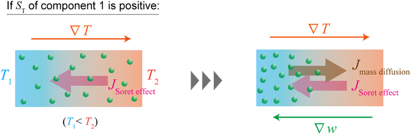
Coupling: mass ↔︎ thermal – Soret / Dufour effects
Coupled flux–force relations
- Mass flux driven by temperature gradient (Soret effect)
- Heat flux driven by concentration gradient (Dufour effect)
Derivation of Soret thermal conductivity please see lecture handwritten notes
![]()
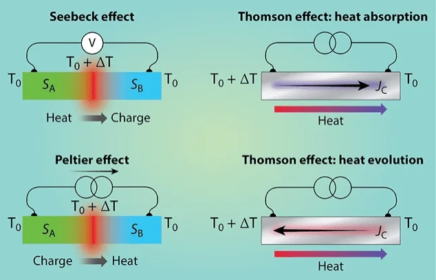
Coupling: charge ↔︎ thermal – Seebeck / Peltier effects
Coupled flux–force relations - Electric current driven by temperature gradient (Seebeck effect) - Heat flux driven by electric field (Peltier effect)
![]()
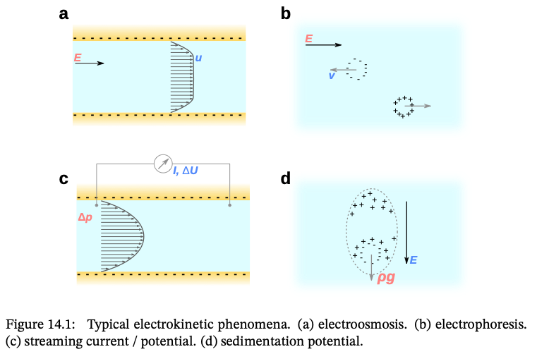
Coupling: charge ↔︎ mass – electrokinetic phenomena
Coupled flux–force relations - Charge and mass transport are interdependent in ionic systems
![]()
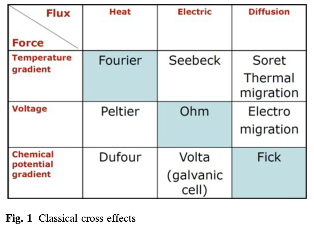
General matrix for coupling effects
Example coupling effect matrix given in J. Phase Equilib. Diffus. 2022 43, 640
![]()
Some additional consequence of Onsager reciprocity
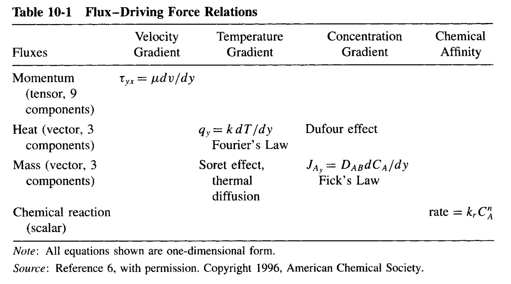
There are some consequences of Onsager’s reciprocity. As Curie’s symmetry principle (1894, Pierre Curie, not Marie) stated, the cause of an effect needs to follow tensor rank selection rule, that:
Flux – Driving Force pair can only be induced when they have the same tensor rank, or differ by 2.
![]()
Tensor rank coupling from Griskey Book 2002
The coupling of momentum-transfer (fluid, 2nd-order) and chemical reaction (0th-order) has only been recently proposed! See J. Chem. Phys. 2022, 157, 084901.
Summary
- Entropy balance equation 👉 solutions for flux of entropy and entropy production
- Entropy production rate 👉 flux of quantity ✖️ driving force
- Flux of quantity 👉 Coefficient ✖️ Driving Force
- Examples of reciprocal relation in transport phenomena
- Brief introduction of diffusion