CHE 318 Lecture 07
Steady State Mass Transfer – Other Geometries
2026-01-19
Recap
- Examples of steady state diffusion
- Applying steady state flux equations to solid and liquid systems
- Examples for several special forms
- weight % and average concentration in liquid
- log mean form of concentration / molar fraction
- pressure - solubility - permeability
Learning outcomes
(Continue from Lecture 06) After this lecture, you will be able to:
- Recall how geometry changes the diffusion area and flux expression.
- Describe approximations used in spherical and non-uniform-area diffusion problems.
- Identify when the stagnant-B formulation applies to spherical evaporation problems.
- Apply pseudo-steady-state analysis to diffusion problems with changing diffusion paths.
- Calculate diffusivities from evaporation data in non-planar geometries.
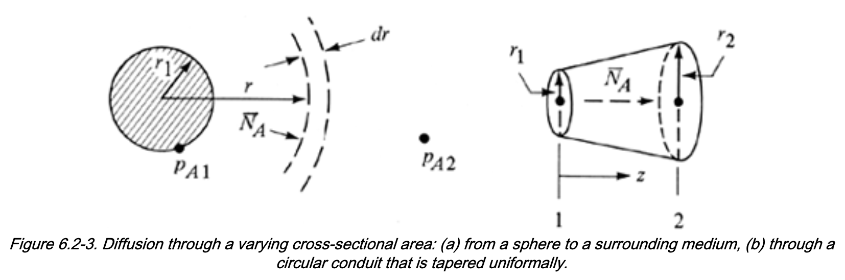
Diffusion through varying cross-sectional area
Steady state mass balance
Many industrial applications involde 1D transport with variable area \(A(z)\), with mass balance:
\[\begin{align} [\mathrm{In}] - [\mathrm{Out}] &= 0 \\ N_{A1} A_1 - N_{A2} A_2 &= 0 \end{align}\]Define the total molar flow rate of A:
\[ \overline{N}_A = N_A \, A(z) \]
At steady state: - \(\overline{N}_A\) is constant - \(N_A\) varies with position if \(A(z)\) (or \(A(r)\)) varies
Applications of variable-area diffusion
This framework can be used to solve diffusion through:
- Sphere
- Cylinder
- Tube with varying diameter
- Any system with a known area function \(A = A(z)\) or \(A=A(r)\)
Key ideas
- Do not solve as simple 1D Cartesian diffusion
- Geometry enters through \(A(z)\)
- Flux adjusts to maintain constant \(\overline{N}_A\)
Case study 1: diffusion through a sphere
Typical physical situations
- Evaporation of a liquid droplet
- Sublimation of a solid organic sphere
Conditions
- Steady state
- Stagnant B (\(N_B = 0\))
- Radial symmetry
Governing equation (stagnant B): use the ODE form, not the full 1D Cartesian solution:
\[\begin{align} N_A &= -\frac{D_{AB}}{RT}\frac{d p_A}{dr} + \frac{p_A}{p_T} N_A \\ N_A\!\left(1 - \frac{p_A}{p_T}\right) &= -\frac{D_{AB}}{RT}\frac{d p_A}{dr} \end{align}\]Stagnant B in a sphere: reformulation
For spherical symmetry, \(N_A(r)\) varies with \(r\) and cannot appear alone in the balance equation L.H.S
Use the constant molar flow rate: \[ \overline{N}_A = N_A(r)\,4\pi r^2 = \text{constant} \]
\[\begin{align} \frac{\overline{N}_A}{4\pi r^2}\,dr &= -\frac{D_{AB}}{RT}\frac{1}{1-p_A/p_T}\,dp_A \end{align}\]Stagnant B in a sphere: final results
\[\begin{align} \boxed{ \frac{\overline{N}_A}{4\pi} \left(\frac{1}{r_1}-\frac{1}{r_2}\right) = \frac{D_{AB}p_T}{RT} \ln\!\left(\frac{p_T-p_{A2}}{p_T-p_{A1}}\right) } \end{align}\]This looks very similar to the 1D stagnant B solution in cartesian coordinates. We can simplify it in several occations.
Stagnant B in a sphere: far-field limit (\(r_2 \gg r_1\))
Special case: \(r_2 \gg r_1\) (often \(r_2 \to \infty\))
Typical examples: - Evaporating liquid droplet - Sublimation of a naphthalene (solid) sphere
From the general spherical stagnant-B result, use the log-mean pressure form:
\[\begin{align} \boxed{ N_{A1} = \frac{D_{AB} p_T}{RT\,p_{Bm}} \left(p_{A1} - p_{A2}\right) } \end{align}\]Where \(N_{A1} = N_A(r=r_1)\). For liquid, another form is often used (considering \(p_{Bm}/p_T \approx 1\) and use \(p = cRT\))
\[\begin{align} \boxed{ N_{A1} = \frac{D_{AB}}{r_1}\left(c_{A1} - c_{A2}\right) } \end{align}\]Spherical diffusion: thin shell limit \(r_1 \approx r_2\)
Special case: thin membrane / shell
\(\Delta r = r_2 - r_1 \ll r_1\)
Approximation: \[ \frac{1}{r_1} - \frac{1}{r_2} \;\approx\; \frac{r_2 - r_1}{r_1^2} \;=\; \frac{\Delta r}{r_1^2} \]
Final result:
\[\begin{align} \boxed{ N_{A1} = \frac{D_{AB}}{RT}\frac{p_T}{p_{Bm}} \frac{(p_{A1}-p_{A2})}{\Delta r} } \end{align}\]This acts like a 1D stagnant-B film with thickness \(\Delta r\)! (See lecture 3 wooclap question.)
Case 2: diffusion through a non-uniform area conduit
Conditions:
- Stagnant B
- Steady state
- Variable radius \(r(z)\)
Assume linear radius profile: \[ r(z) = r_1 + \frac{(r_2-r_1)}{(z_2-z_1)}(z-z_1) \]
Use the ODE form with \(\dot N_A = N_A(z)\,A(z)\) and \(A(z)=\pi r(z)^2\):
\[\begin{align} \frac{\dot N_A}{\pi}\int_{z_1}^{z_2}\frac{dz}{\left[r(z)\right]^2} &= -\frac{D_{AB}}{RT}\int_{p_{A1}}^{p_{A2}} \frac{dp_A}{1-p_A/p_T} \end{align}\]Can you solve for \(N_{A1}\)?
Examples for Pseudo Steady State (P.S.S)
Example 1: diffusion through stagnant B with changing path length
Adapted from Geankoplis 6.2-3
Water vapor diffuses through a stagnant gas in a narrow vertical tube, dry air is constantly blown at the top of tube.
At time \(t\), the liquid level is a distance \(z\) from the tube top (i.e., the diffusion path length is \(z\)).
As diffusion proceeds, the liquid level drops slowly, so \(z\) increases with time. The liquid has density \(\rho_A\), and molecular weight \(M_A\)
- Derive an expression for the time \(t_F\) required for the level to drop such that the diffusion path length changes from \(z=z_0\) at \(t=0\) to \(z=z_F\) at \(t=t_F\).
Example 1: solutions
Tip
- Use pseudo steady-state assumption
- \(N_A\) change over time!
Answer \[ t_F = \frac{\rho_A (z_F^2 - z_0^2) RT p_{Bm}}{2 D_{AB} M_A p_{T}} \frac{1}{(p_{A1} - p_{A2})} \]
Example 2: determine \(D_{AB}\) through evaporation
Adapted from Griskey 10-2
Sample setup as example 4, a vertical tube of diameter \(D=0.01128\) m contains a liquid volatile species \(A\) (chloropicrin, \(CCl_3NO_2\)) evaporating into stagnant air (\(B\)) at 1 atm. The gas-phase diffusion of \(A\) occurs through the air column above the liquid surface.
At \(t=0\), the distance from the tube top to the liquid surface is \(z_0 = 0.0388\) m, after \(t=1\) day, the distance is \(z_1 = 0.0412\) m.
- Vapor pressure at the interface: \(p_{A1} = 3178.3\) Pa
- Liquid density: \(\rho_A = 1650\) kg/m\(^3\)
- Molecular weight: \(M_A = 164.39\) kg/kmol
- Use your expression from example 4, determine the binary diffusivity \(D_{AB}\) of \(A\) in air.
Example 2: solutions
Tip
Pseudo steady state solution and assuming \(N_A=\text{const}\) solution differ very little. Why?
Answer:
- Pseudo-steady state: \(D_{AB} = 8.56\times{}10^{-6}\ \text{m}^2/\text{s}\)
- \(N_A\) constant: \(D_{AB} = 8.75\times{}10^{-6}\ \text{m}^2/\text{s}\) (\(+2.2\%\) error)
Example 3: P.S.S for diffusion through sphere
Adapted from Geankoplis Ex 6.2-4
A sphere of naphthalene having a radius of 2.0 mm is suspended in a large volume of still air at 318 K and \(1.01325 \times{}10^5\) Pa (1 atm). The surface temperature of the naphthalene can be assumed to be at 318 K and its vapor pressure at 318 K is 0.555 mm Hg. The \(D_{AB}\) of naphthalene in air at 318 K is \(6.92\times{}10^{−6}\ \text{m}^2/\text{s}\).
- Calculate the rate of evaporation of naphthalene from the surface.
- Write the expression for the time \(t_F\) to evaporate a sphere from radius \(r_0\) to \(r_F\). The solid density for naphthalene is \(\rho\) and molecular weight is \(M_A\).
- What is the \(t_F\) value when the sphere is completely evaporated?
Example 3: solutions
Tip
Similar setup as example 5. \(N_A\) is time-dependent
Answer:
- \(N_A = 9.68\times{}10^{-8}\ \text{kg mol}/\text{m}^2/\text{s}\)
- Expression for \(t_F{r=r_F}\): \[ t_F(r=r_F) = \frac{\rho RT p_{Bm}}{2 M_A D_{AB} p_T} \frac{1}{(p_{A1} - p_{A2})} (r_0^2 - r_F^2) \]
- Expression for \(t_F{r=0}\): \[ t_F(r=0) = \frac{\rho RT p_{Bm} r_0^2}{2 M_A D_{AB} p_T} \frac{1}{(p_{A1} - p_{A2})} \]
Compare the solutions with Example 4. We can also measure the diffusivity of volatile organic molecules using the sphere evaporation methods!
Summary
- Solving diffusion through varying cross-section
- Pseudo-steady state solutions to diffusion-evaporation problems