CHE 318 Lecture 09
Introduction to Unsteady State Mass Transfer
2026-01-23
Recap
- Solving examples with pseudo steady state assumption
- Conclusion of steady state mass transfer
Learning outcomes
After this lecture, you will be able to:
- Recall the difference between steady-state and unsteady-state mass transfer problems.
- Derive transient mass-balance and flux equations for diffusion systems.
- Identify accumulation and generation terms in typical transport models.
- Analyze time-dependent concentration profiles in unsteady diffusion problems.
What is unsteady-state mass transfer?
![]()
- Concentration varies with time \(\partial c/\partial t \neq 0\)
- Accumulation term is non-zero \(\text{[Acc]} \neq 0\)
- Requires time-dependent mass balances
- Common in transient diffusion, start-up, and response problems
- More general than S.S.
Governing equation for U.S.S M.T.
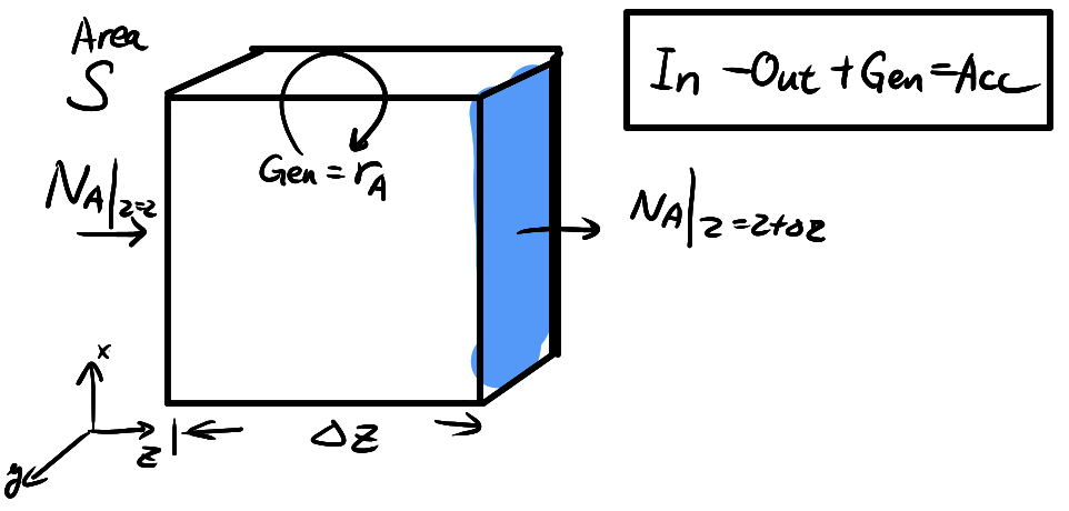
Consider a control volume in 1D transport, the mass balance equation becomes
\[\begin{align*}
\text{[Acc]} &= \text{[In]} - \text{[Out]} + \text{[Gen]} \\
S \Delta z \frac{\partial c_A}{\partial t}
&= S (N_A \vert_{z=z} - N_A \vert_{z=z+\Delta z}) + \text{[Gen]} S \Delta z \\
\frac{\partial c_A}{\partial t}
&=
-\frac{\partial N_A(z)}{\partial z}\vert_z + r_{A}
\end{align*}\]
where \(r_{A}\) is the generation rate for A (e.g. local reaction). This is the governing equation for all time-dependent mass transfer!
Comparison between flux equation and mass balance
Flux equation
\[\begin{align*}
N_A = J_{Az}^* + x_A(N_A + N_B)
\end{align*}\]
- Amount of material moved in and out of the control volume
- \(J_{Az}^*\): Fick’s first law of diffusion
- Can be used for S.S (\(d N_A/dz = 0\)) and U.S.S
Mass balance eq
\[\begin{align}
\frac{\partial c_A}{\partial t} = - \frac{\partial N_A}{\partial x} + r_A
\end{align}\]
- Change of local \(c_A\) over time
- Need flux equation solution first
- Can be used for S.S (\(\frac{\partial c_A}{\partial t} = 0\)) and U.S.S.
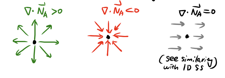
Mass balance: extension to 3D
![]()
Illustration of divergence
\[\begin{align}
\frac{\partial c_A}{\partial t}
&= r_A
- \frac{\partial N_{Ax}}{\partial x}
- \frac{\partial N_{Ay}}{\partial y}
- \frac{\partial N_{Az}}{\partial z} \\
&= r_A - \nabla \cdot \vec{N}_A
\end{align}\]
- \(\nabla \cdot\) is the divergence operator (not \(\Delta\), not gradient!)
- \(\vec{N}_A\) is generally a 3D vector field
Dissecting the general equation for mass balance
\[\begin{align*}
r_A - \frac{\partial c_A}{\partial t}
&= \nabla \cdot \left[\vec{J}_{A}^{*} + x_A(\vec{N}_A + \vec{N}_B) \right] \\
&= \nabla \cdot \left[\vec{J}_{A}^{*} + c_A \vec{v}_m \right] \\
&= \nabla \cdot \left[ -D_{AB} \nabla c_A + c_A \vec{v}_m \right]
\end{align*}\]
- We have fluid velocity \(\vec{v}_m\) on the R.H.S
- \(\nabla \cdot\) creates more nonlinear terms
- Do we know \(N_A\) and \(N_B\) relation?
- In general this is hard to solve (coupling fluid with mass transfer)
- Often interested in several limiting cases
Special cases of unsteady-state mass transfer
- Case 1: EMCD for gases at constant \(p_T\), \(r_A = 0\) (Fick’s second law)
- There is no negative sign in Fick’s second law!
\[\begin{align}
\frac{\partial c_A}{\partial t}
&=
D_{AB}\nabla^2 c_A
\end{align}\]
- Case 2: Constant \(D_{AB}\)
\[\begin{align*}
\frac{\partial c_A}{\partial t}
&=
D_{AB}\nabla^2 c_A
- c_A \nabla \cdot \vec{v}_m
- \vec{v}_m \cdot \nabla c_A
+ r_A
\end{align*}\]
- Case 3: Constant \(\rho\) and \(D_{AB}\) (e.g. incompressible liquids)
\[\begin{align}
\frac{\partial c_A}{\partial t}
&=
D_{AB}\nabla^2 c_A
- \vec{v}_m \cdot \nabla c_A
+ r_A
\end{align}\]
where \(\nabla \cdot \vec{v}_m = 0\)
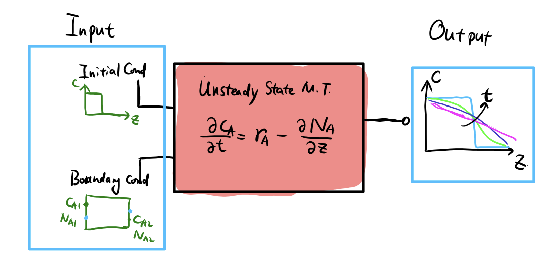
Unsteady state mass transfer: calculation overview
![]()
A “solver engine” for unsteady state mass transfer
Summary
- Unsteady state mass transfer governing equation
- Step-by-step solution to diffusion through stagnant B
- Diffusion and reaction system setup