---
title: "CHE 318 Lecture 09"
subtitle: "Introduction to Unsteady State Mass Transfer"
author: "Dr. Tian Tian"
date: "2026-01-23"
format:
html: {}
revealjs:
output-file: slides.html
pdf:
output-file: L09.pdf
---
::: {.content-visible when-format="html" unless-format="revealjs"}
::: {.callout-note}
- Slides 👉 [Open presentation🗒️](./slides.html)
- PDF version of course note 👉 [Open in pdf](./L09.pdf)
- Handwritten notes 👉 [Open in pdf](./public/L09_annotated.pdf)
:::
:::
## Recap {.center}
- Solving examples with pseudo steady state assumption
- Conclusion of steady state mass transfer
## Learning outcomes {.center}
After this lecture, you will be able to:
- **Recall** the difference between steady-state and unsteady-state mass transfer problems.
- **Derive** transient mass-balance and flux equations for diffusion systems.
- **Identify** accumulation and generation terms in typical transport models.
- **Analyze** time-dependent concentration profiles in unsteady diffusion problems.
## What is unsteady-state mass transfer?
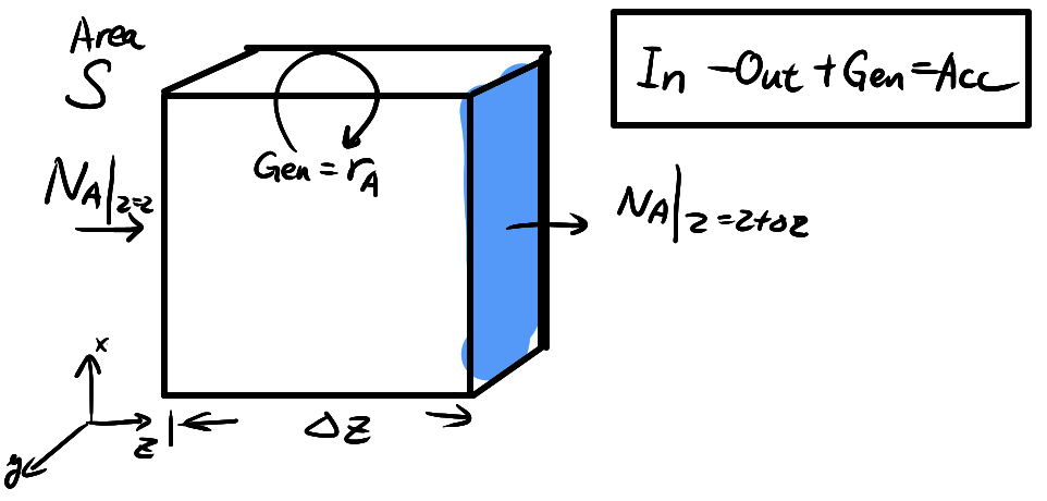{width="65%" .center}
```{=tex}
\text{[In]} - \text{[Out]} + \text{[Gen]} = \text{[Acc]}
```
- Concentration varies with time $\partial c/\partial t \neq 0$
- Accumulation term is non-zero $\text{[Acc]} \neq 0$
- Requires time-dependent mass balances
- Common in transient diffusion, start-up, and response problems
- **More general** than S.S.
## Governing equation for U.S.S M.T.
Consider a control volume in 1D transport, the mass balance equation becomes
```{=tex}
\begin{align*}
\text{[Acc]} &= \text{[In]} - \text{[Out]} + \text{[Gen]} \\
S \Delta z \frac{\partial c_A}{\partial t}
&= S (N_A \vert_{z=z} - N_A \vert_{z=z+\Delta z}) + \text{[Gen]} S \Delta z \\
\frac{\partial c_A}{\partial t}
&=
-\frac{\partial N_A(z)}{\partial z}\vert_z + r_{A}
\end{align*}
```
where $r_{A}$ is the generation rate for A (e.g. local reaction).
This is the governing equation for all time-dependent mass transfer!
## Comparison between flux equation and mass balance
:::{.columns}
:::{.column width="50%"}
#### Flux equation
```{=tex}
\begin{align*}
N_A = J_{Az}^* + x_A(N_A + N_B)
\end{align*}
```
- Amount of material moved **in** and **out** of the control volume
- $J_{Az}^*$: Fick's first law of diffusion
- Can be used for S.S ($d N_A/dz = 0$) and U.S.S
:::
:::{.column width="50%"}
#### Mass balance eq
```{=tex}
\begin{align}
\frac{\partial c_A}{\partial t} = - \frac{\partial N_A}{\partial x} + r_A
\end{align}
```
- Change of local $c_A$ over time
- Need flux equation solution first
- Can be used for S.S ($\frac{\partial c_A}{\partial t} = 0$) and U.S.S.
:::
:::
## Mass balance: extension to 3D
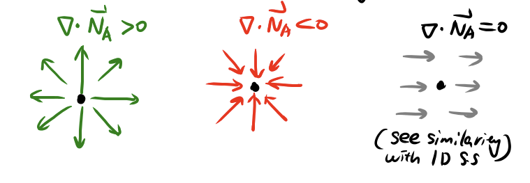{width="75%" .center}
```{=tex}
\begin{align}
\frac{\partial c_A}{\partial t}
&= r_A
- \frac{\partial N_{Ax}}{\partial x}
- \frac{\partial N_{Ay}}{\partial y}
- \frac{\partial N_{Az}}{\partial z} \\
&= r_A - \nabla \cdot \vec{N}_A
\end{align}
```
- $\nabla \cdot$ is the **divergence** operator (not $\Delta$, not gradient!)
- $\vec{N}_A$ is generally a 3D vector field
---
## How to analyze a U.S.S problem
Unsteady state mass transfer is not intimidating if you follow these steps
1. Draw the scheme
2. Write down the **mass balance** equation ([In] - [Out] + [Gen] = [Acc])
3. Identify the [Gen] and [Acc] terms
4. Choose proper **flux equations** for [In] and [Out] terms
5. Solving analytically or numerically.
---
## Dissecting the general equation for mass balance
```{=tex}
\begin{align*}
r_A - \frac{\partial c_A}{\partial t}
&= \nabla \cdot \left[\vec{J}_{A}^{*} + x_A(\vec{N}_A + \vec{N}_B) \right] \\
&= \nabla \cdot \left[\vec{J}_{A}^{*} + c_A \vec{v}_m \right] \\
&= \nabla \cdot \left[ -D_{AB} \nabla c_A + c_A \vec{v}_m \right]
\end{align*}
```
- We have fluid velocity $\vec{v}_m$ on the R.H.S
- $\nabla \cdot$ creates more nonlinear terms
- Do we know $N_A$ and $N_B$ relation?
- In general this is hard to solve (coupling fluid with mass transfer)
- Often interested in several limiting cases
## Special cases of unsteady-state mass transfer
- Case 1: EMCD for gases at constant $p_T$, $r_A = 0$ (Fick’s second law)
- There is **no negative sign** in Fick's second law!
```{=tex}
\begin{align}
\frac{\partial c_A}{\partial t}
&=
D_{AB}\nabla^2 c_A
\end{align}
```
- Case 2: Constant $D_{AB}$
```{=tex}
\begin{align*}
\frac{\partial c_A}{\partial t}
&=
D_{AB}\nabla^2 c_A
- c_A \nabla \cdot \vec{v}_m
- \vec{v}_m \cdot \nabla c_A
+ r_A
\end{align*}
```
- Case 3: Constant $\rho$ and $D_{AB}$ (e.g. incompressible liquids)
```{=tex}
\begin{align}
\frac{\partial c_A}{\partial t}
&=
D_{AB}\nabla^2 c_A
- \vec{v}_m \cdot \nabla c_A
+ r_A
\end{align}
```
where $\nabla \cdot \vec{v}_m = 0$
## What exactly do we solve?
For U.S.S M.T, we typically need
1. Governing equation (PDE) from any limiting case
2. Initial conditions $c_A(z, t=0)$
3. Boundary conditions (B.C.)
- Dirichlet B.C. (e.g. $c_A(z=0) = c_0$)
- Neumann B.C. (e.g. $N_A(z=0) = N_{A0}$, constant flux)
4. Solving analytically or numerically
5. Get $c_A(z, t)$, $x_A(z, t)$, $N_A(x, t)$
6. Steady-state solutions often means $c_A(z, t\to \infty)$
## Unsteady state mass transfer: calculation overview
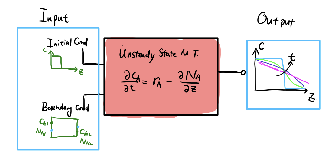{width="85%"}
<!-- ## B.C. Case 1. Concentration at surfaces -->
<!-- {width="55%"} -->
<!-- - Interface can be gas|liquid, liquid|solid, gas|solid -->
<!-- - Often assuming equilibrium -->
<!-- $$ -->
<!-- c_{A}\vert_{\text{surf}} = c_{As}\qquad\text{eq. solubility} -->
<!-- $$ -->
<!-- ## B.C. Case 2: Chemical Reactions -->
<!-- {width="55%"} -->
<!-- ```{=tex} -->
<!-- \begin{align} -->
<!-- N_A\big|_{\text{surf}} = \nu_A\, r_A -->
<!-- \end{align} -->
<!-- ``` -->
<!-- - Surface reaction couples mass transfer and kinetics -->
<!-- - Molar flux at surface determined by reaction rate -->
<!-- - Generally Neumann boundary -->
<!-- - $\nu_A$: stoichiometric ratio -->
<!-- ## B.C. Case 3: Constant Flux -->
<!-- {width="55%"} -->
<!-- - In many cases the flux $N_{A, \text{surf}}$ or $N_{B, \text{surf}}$ can be constant. -->
<!-- - E.g. inpenetratable surface to stagnant gas $N_{B, \text{surf}} = 0$ -->
<!-- - **Does not** mean $N_{A}(z)$ or $N_B(z)$ elsewhere is constant! -->
<!-- ## U.S.S Example 1: Diffusion Through Stagnant B -->
<!-- We have seen in previous examples how to solve the molar flux of -->
<!-- liquid evaporating into stagnant air. Let's see the same system but in unsteady state. -->
<!-- **Question**: liquid methanol (A) evaporates inside stagnant air (B) -->
<!-- inside a vertical tube at constant temperature $T$ and pressure -->
<!-- $p_T$. At the vent of the system dry air is continuous blown. Plot the -->
<!-- molar fraction $x_A$ as a function of $z$ and time $t$. Assume the liquid level is $z_0$ away from the vent and does not change during the evaporation process. -->
<!-- ## Step 1: Species Mass Balance (Unsteady, 1D) -->
<!-- For a differential slice $A\,dz$, write the mass balance -->
<!-- ```{=tex} -->
<!-- \begin{align} -->
<!-- \text{[IN]} - \text{[OUT]} &= \text{[ACC]} \\ -->
<!-- A N_A \vert_{z=z} - A N_A \vert_{z=z+\Delta z} -->
<!-- &= \frac{\partial}{\partial t}\left(A\,dz\,c_A\right) \\ -->
<!-- -\frac{\partial N_A}{\partial z} = \frac{\partial c_A}{\partial t} -->
<!-- \end{align} -->
<!-- ``` -->
<!-- We would have $\frac{\partial c_B}{\partial t} = -\frac{\partial N_B}{\partial z}$ -->
<!-- ## Step 2: Couple With Flux Equation -->
<!-- This is a diffusion through stagnant B case, we can directly write -->
<!-- ```{=tex} -->
<!-- \begin{align} -->
<!-- N_A(z, t) = -c_T D_{AB}\frac{\partial x_A(z, t)}{\partial z} + x_A \left[N_A(z, t) + N_B(z, t)\right] -->
<!-- \end{align} -->
<!-- ``` -->
<!-- - Can we use $N_B=0$ in this case? -->
<!-- - **No**, $N_B$ changes by $z, t$! -->
<!-- - $N_B=0$ only at $z=0$ (liquid interface) -->
<!-- - **Do not** write the steady state $N_A$ solution! -->
<!-- ## Step 3: Conservation Equations -->
<!-- Generally, we still need to know the relation between $N_A$ and $N_B$ -->
<!-- to solve the mass-balance-flux equations. -->
<!-- The total concentration $c_T=c_A + c_B$ is conserved, therefore we have constrains -->
<!-- ```{=tex} -->
<!-- \begin{align} -->
<!-- \text{[In]}_{T} - \text{[Out]}_{T} &= 0 \\ -->
<!-- \text{[In]}_A - \text{[Out]}_A &= -\text{[In]}_B + \text{[Out]}_B \\ -->
<!-- \frac{\partial N_A(z, t)}{\partial z} &= -\frac{\partial N_B(z, t)}{\partial z} -->
<!-- \end{align} -->
<!-- ``` -->
<!-- ## Step 4: Boundary Conditions -->
<!-- Boundary conditions (Left, Right, any time) -->
<!-- - $x_A(0, t) = x_{A0}$ (equilibrium vapor fraction) -->
<!-- - $x_A(L, t) = 0$ (dry air) -->
<!-- - $N_B(0, t) = 0$ (No-flux boundary for B) -->
<!-- The last B.C for $N_B(0, t)$ gives: -->
<!-- ```{=tex} -->
<!-- \begin{align} -->
<!-- N_A(0, t) = -\frac{c_T D_{AB}}{1 - x_{A0}}\frac{\partial x_A(0, t)}{\partial z} -->
<!-- \end{align} -->
<!-- ``` -->
<!-- ## Step 5: Final solution -->
<!-- - Unsteady state flux equation (stagnant B) -->
<!-- ```{=tex} -->
<!-- \begin{align} -->
<!-- N_A = -c_T D_{AB} \frac{\partial x_A}{\partial z} -->
<!-- + x_A \left[ \frac{-c_T D_{AB}}{1 - x_{A0}} \frac{\partial x_{A}}{\partial z}\big\vert_{z=0} \right] -->
<!-- \end{align} -->
<!-- ``` -->
<!-- - Governing equation for diffusion through stagnant B, unsteady state: -->
<!-- ```{=tex} -->
<!-- \begin{align} -->
<!-- \frac{\partial x_A}{\partial t} -->
<!-- = c_T D_{AB} \frac{\partial^2 x_A}{\partial z^2} -->
<!-- + \left[ \frac{-c_T D_{AB}}{1 - x_{A0}} \frac{\partial x_{A}}{\partial z}\big\vert_{z=0} \right] \frac{\partial x_A}{\partial z} -->
<!-- \end{align} -->
<!-- ``` -->
<!-- - Analytical solution exists, but numerical solution is more convenient -->
<!-- ## U.S.S Example 2: Transport Through A Catalyst Wall -->
<!-- **Question**: A gas mixture containing species A flows through a -->
<!-- cylindrical conduit of diameter $D$ with a constant mean velocity -->
<!-- $v_m$. A porous catalytic wall of thickness $\Delta z$ is located at a -->
<!-- fixed axial position inside the conduit. Inside the catalyst region, -->
<!-- species A is consumed by a first-order surface reaction: -->
<!-- $$ -->
<!-- r = -->
<!-- k'(c_{A,s} - c_A) -->
<!-- $$ -->
<!-- Assume: -->
<!-- - surface concentration on catalyst, $c_{A,s}$ is constant -->
<!-- - uniform properties in the radial direction -->
<!-- - constant $T$, $P$, and physical properties -->
<!-- - no reaction outside the catalyst region -->
<!-- ## Step 1: Mass Balance -->
<!-- Consider a differential gas-phase control volume of thickness $\Delta z$ that intersects the catalytic wall. -->
<!-- ```{=tex} -->
<!-- \begin{align} -->
<!-- \text{In} - \text{Out} + \text{Generation} &= \text{Accumulation} \\ -->
<!-- \\ -->
<!-- \frac{\pi D^2}{4} -->
<!-- \left( -->
<!-- N_A\big|_{z} -->
<!-- - -->
<!-- N_A\big|_{z+\Delta z} -->
<!-- \right) -->
<!-- + -->
<!-- \pi D\,\Delta z\,k\,(c_{A,s}-c_A) -->
<!-- &= -->
<!-- \frac{\pi D^2}{4}\, -->
<!-- \frac{\partial C_A}{\partial t} \\ -->
<!-- -\frac{\partial N_A}{\partial z} -->
<!-- + -->
<!-- \frac{4k}{D}\,(c_{A,s}-c_A) -->
<!-- = -->
<!-- \frac{\partial c_A}{\partial t} -->
<!-- \end{align} -->
<!-- ``` -->
<!-- ## Step 2: Coupling With Flux Equation -->
<!-- Use the convection–diffusion flux (constant $v_m$): -->
<!-- ```{=tex} -->
<!-- \begin{align} -->
<!-- N_A -->
<!-- = -->
<!-- -\,D_{AB}\,\frac{\partial c_A}{\partial z} -->
<!-- + -->
<!-- c_A\,v_m -->
<!-- \end{align} -->
<!-- ``` -->
<!-- When $v_m$ is constant, differentiate over $N_A$ becomes: -->
<!-- ```{=tex} -->
<!-- \begin{align} -->
<!-- \frac{\partial N_A}{\partial z} -->
<!-- = -->
<!-- -\,D_{AB}\,\frac{\partial^2 c_A}{\partial z^2} -->
<!-- + -->
<!-- v_m\,\frac{\partial c_A}{\partial z} -->
<!-- \qquad (v_m=\text{const}) -->
<!-- \end{align} -->
<!-- ``` -->
<!-- ## Step 3: General Equation for M.T + Surface Reaction -->
<!-- ```{=tex} -->
<!-- \begin{align} -->
<!-- \frac{\partial c_A}{\partial t} -->
<!-- &= -->
<!-- -\left( -->
<!-- -\,D_{AB}\,\frac{\partial^2 c_A}{\partial z^2} -->
<!-- + -->
<!-- v_m\,\frac{\partial c_A}{\partial z} -->
<!-- \right) -->
<!-- + -->
<!-- \frac{4k}{D}\,(c_{A,s}-c_A) \\ -->
<!-- &= -->
<!-- D_{AB}\,\frac{\partial^2 c_A}{\partial z^2} -->
<!-- - -->
<!-- v_m\,\frac{\partial c_A}{\partial z} -->
<!-- + -->
<!-- \frac{4k}{D}\,(c_{A,s}-c_A) -->
<!-- \end{align} -->
<!-- ``` -->
<!-- Need: -->
<!-- - initial condition $c_A(z,0)$ -->
<!-- - boundary conditions at $z=0$ and $z=L$ -->
<!-- Solve: -->
<!-- - analytical (special cases) -->
<!-- - numerical integration (finite difference) -->
## Summary
- Unsteady state mass transfer governing equation
- Step-by-step solution to diffusion through stagnant B
- Diffusion and reaction system setup


