CHE 318 Lecture 17
Dimensionless Numbers In Mass Transfer
2026-02-13
Learning outcomes
After this lecture, you will be able to:
- Recall the physical meaning of key dimensionless numbers in mass transfer.
- Describe how Reynolds, Schmidt, and Sherwood numbers correlate mass transfer behavior.
- Identify suitable dimensionless correlations for different flow geometries.
Recap: boundary layer theory
The global mass transfer coefficient in a tube:
\[\begin{align} k_c' = \frac{0.664 D_{AB}}{L} N_{Re}^{0.5} N_{Sc}^{1/3} \end{align}\]- \(N_{Re}\): Reynolds number
- \(N_{Sc}\): Schmidt number
Why do we need these dimensionless numbers?
- Expressing fluxes using \(k\) coefficients are easy
- But do we need to measure \(k\) for each system specifically?
- Of course NO!
- We can correlate the values of \(k\) measured in different geometries, velocities using dimensionless numbers
- Similar treatment exists in heat and momentum (fluid) transfer
Dimensionless numbers in mass transfer
General form: \(N_{\text{name}} = \dfrac{\text{Scale of effect 1}}{\text{Scale of Effect 2}}\)
Schmidt number (ratio between momentum diffusivity and molecular diffusivity)
- Sherwood number (ratio between convective mass transfer and molecular mass transfer)
- Reynolds number (ratio between kinetic vs viscous forces of fluid flow)
- \(L\): characteristic length of system
- Location specific \(N_{\text{Re}, x}\) also used
Meaning of dimensionless numbers – \(N_{Re}\)
- \(N_{Re}\): laminar flow vs turbulent flow
- Varies with characteristic length \(L_D\) (diameter for a pipe)
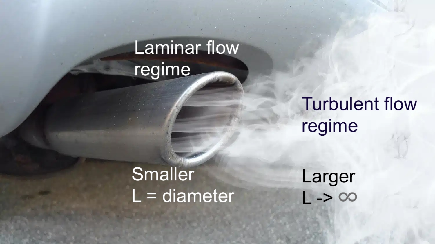
\(N_{Re}\) for exhaust pipe
How are \(k_c'\) correlated by dimensionless numbers?
- Idea: mass transfer in flowing fluid described by \(v\), \(\rho\), \(\mu\), \(c\), \(D_{AB}\) and geometry (characteristic length \(L\))
- The combinations of these properties –> dimensionless number groups (\(N_{\text{Sc}}\), \(N_{\text{Sh}}\), \(N_{\text{Re}}\))
- The Chilton-Colburn \(j\)-factor analog has most successful use in mass transfer
- \(f\) is the Fanning Friction Factor (can be found in table)
General procedure to calculate \(k_c'\)
Calculate Reynolds number \(N_{Re}\) from fluid properties + geometry
Determine flow regime (liquid)
- \(N_{Re} < 2100\) → laminar flow
- \(N_{Re} \ge 2100\) → turbulent flow
- Evaluate friction factor \(f\)
- Laminar flow:
\[ f = \frac{16}{N_{Re}} \] - Turbulent flow:
\[ f = \frac{\tau_s}{\tfrac12 \rho v^2},\qquad \tau_s = \frac{\Delta P_f\,\pi R^2}{2\pi R\,\Delta L} \]
Compute mass-transfer \(j\)-factor
\[ j_D = \frac{f}{2} \]Obtain mass-transfer coefficient
\[ k_c' = j_D\,v_{av}\,N_{Sc}^{-2/3} \]
Use of empirical mass transfer laws
- In many systems, flux and / or concentration profiles become hard to have simple form
- Luckily we can simplify typical mass transfer problems as different geometries
- Cyliner / Pipe
- Parallel plates
- Flow around sphere
- Packed bed
- We will show a few case studies for different geometries
- Dimensionless numbers (\(N_{Re}\), \(N_{Sc}\), \(N_{Sh}\)) help determine governing equations
Case 1: mass transfer for flow inside pipes
- Usually use the Linton & Sherwood chart
- Valid for gas / liquid in both laminar & turbulent regimes
Flow inside pipe: chart
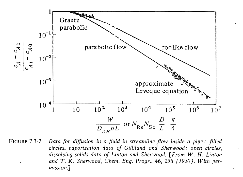
Flow inside pipes: solution procedure
- Governing dimensionless quantity:
- If gas 👉 use the “rodlike flow” line
- If liquid, distinguish 2 cases
- parabolic flow (\(N_{Re} < 2100;\ \frac{W}{D_{AB}\rho L} > 400\))
- turbulent flow (\(N_{Re} > 2100;\ 0.6 < N_{Sc} < 3000\))
Flow inside pipes: solution for liquid
Parabolic flow
\[\begin{align} \frac{c_A - c_{A,s}}{c_{A,i} - c_{A,s}} &= 5.5 \left[ \frac{W}{D_{AB}\,\rho\,L} \right]^{-\tfrac{2}{3}} \end{align}\]\(c_A\): exit concentration
\(c_{A,i}, c_{A,s}\): inlet & surface concentration
\(W\): flow rate in (kg/s)
\(k_c'\) can be calculated by \(j_D\)
Turbulent flow
\[\begin{align} N_{Sh} &= k_c'\left(\frac{D}{D_{AB}}\right) \\ &= \frac{k_c\,p_{BM}}{P} \left(\frac{D}{D_{AB}}\right) \\ &= 0.023 \left(\frac{\rho D v}{\mu}\right)^{0.83} \left(\frac{\mu}{\rho D_{AB}}\right)^{0.33} \\ &= 0.023\, N_{Re}^{0.83}\, N_{Sc}^{0.33} \end{align}\]- Similar to the \(j_D\) analog
- Just need \(N_{Re}\) and \(N_{Sc}\) to determine \(k_c'\)
- Characteristic length \(D\) is pipe diameter!
Case 2: flow past parallel plates
- Can be used for gases or evaporation of liquid
- Distinguished between laminar & turbulent flow
- \(N_{Re}\) regime cutoff different in gas & liquid!
- Characteristic length \(L\): length of plate in flow direction
Flow past parallel plates: results
Laminar flow (\(N_{Re} < 15,000\))
\[\begin{align} j_D &= 0.664 N_{Re, L}^{-0.5} \\ \frac{k_c' L}{D_{AB}} &= 0.664 N_{Re, L}^{0.5} N_{Sc}^{1/3} \end{align}\]- This follows our derivation of boundary layer theory
Turbulent flow
- Gas: \(15,000 < N_{Re}< 300,000\)
- Liquid: \(600 < N_{Re}< 50,000\)
Case 3: flow past single sphere
- Frequent geometry in particle solutions
- Low Reynolds regime 👉 solution for stagnant diffusion on spherical surface
- High Reynolds regime 👉 correct \(N_{Sh}\) and back calculate \(k_c'\)
Flow past single sphere: results
Low Reynolds (\(N_{Re} < 2\))
\[\begin{align} N_A &= \boxed{\frac{2 D_{AB}}{D_p}} (c_{A1} - c_{A2}) \\ &= k_c (c_{A1} - c_{A2}) \\ &= \frac{k_c'}{x_{Bm}}(c_{A1} - c_{A2}) \\ \end{align}\]- For \(x_{Bm} \approx 1\), we have:
\[ k_c' = \frac{2D_{AB}}{D_p} \]
- Sherwood number: \(N_{Sh} = 2\)
High Reynolds (\(N_{Re} > 2\))
- Gas:
- Liquid:
- Back calculate \(k_c' = N_{Sh} \frac{D_{AB}}{D_p}\)
Case 4: mass transfer for packed beds
- Very common geometry for chemical engineering
- Adsorption and desorption through solid particles (gases and liquids)
- Catalytic processes with very large surface area
- Geometry characteristics: void fraction \(\varepsilon\): \[
\varepsilon
= \frac{\text{void space}}{\text{total space}}
= \frac{\text{void space}}{\text{void space} + \text{solid space}}
\]
- Typically \(0.3 < \varepsilon < 0.5\)
- Void fraction is difficult to measure experimentally
Correlation equations in packed bed
Correlation 1, applicable to:
- gase with \(10 < N_{Re} <10,000\)
- liquid with \(10 < N_{Re} < 1500\)
- \(D_p\): (average) particle diameter
- \(v’\): superficial velocity in the tube without packing
Correlation equations in packed bed (II)
Correlation 2, applicable to:
- liquid with \(0.0016 < N_{Re} < 55\), \(165 < N_{Sc} < 70000\)
- liquid with \(55 < N_{Re} < 1500\), \(165 < N_{Sc} < 10690\)
Correlation equations in packed bed (III)
Correlation 3, applicable to fluidized beds
- \(10 < N_{Re} < 4000\) (gas & liquid)
- \(1 < N_{Re} < 10\) (liquid only)
Packed bed calculation steps
- Known value from operational column: \(\varepsilon\), \(V_b\) (total volume), \(D_p\), \(D_{AB}\), \(\mu\), \(\rho\), etc.
- Depend on the operational range, calculate \(N_{Re}\), \(N_Sc\) 👉 choose the equation for \(j_D\)
- Obtain \(k_c\) from \(j_D\) value
- Calculate flux \(N_A\)
- Estimate effective area \(A_{\text{eff}}\) inside the columne 👉 \(\overline{N}_A = A_{\text{eff}} N_A\)
Caveats in packed bed problems (1)
- Estimate the effective area?
- First calculate the effective surface area per volume \(a\) then \(A_{\text{eff}}\)
Caveats in packed bed problems (2)
- Use log-mean driving force (see Lecture 21)
where
- \(c_{A, i}\): surface concentration
- \(c_{A1}, c_{A2}\): in- and outlet concentrations
Caveats in packed bed problems (3)
- Mass-flow balance
where \(Q\) is the volumetric flow rate (unit m\(^3\)/s).
These equations will give rise to solving the flow in packed bed problem.
Summary
- Dimensionless numbers can be used to correlate mass transfer problems in different flow rate, dimension etc
- Typically, start with a known geometry (pipe? parallel plate? sphere? packed bed?)
- Find the correlation with dimensionless numbers \(N_{Re}\), \(N_{Sc}\)
- Calculate the final mass transfer rate