CHE 318 Lecture 17
Dimensionless Numbers In Mass Transfer
- Slides 👉 Open presentation🗒️
- PDF version of course note 👉 Open in pdf
- Handwritten notes 👉 Open in pdf
This lecture contains the overview of dimensionless number relation to mass transfer coefficients. Detailed discussions will be included in Lecture 18, Lecture 19, Lecture 20 and Lecture 21
Learning outcomes
After this lecture, you will be able to:
- Recall the physical meaning of key dimensionless numbers in mass transfer.
- Describe how Reynolds, Schmidt, and Sherwood numbers correlate mass transfer behavior.
- Identify suitable dimensionless correlations for different flow geometries.
Recap: boundary layer theory
The global mass transfer coefficient in a tube:
\[\begin{align} k_c' = \frac{0.664 D_{AB}}{L} N_{Re}^{0.5} N_{Sc}^{1/3} \end{align}\]- \(N_{Re}\): Reynolds number
- \(N_{Sc}\): Schmidt number
Why do we need these dimensionless numbers?
- Expressing fluxes using \(k\) coefficients are easy
- But do we need to measure \(k\) for each system specifically?
- Of course NO!
- We can correlate the values of \(k\) measured in different geometries, velocities using dimensionless numbers
- Similar treatment exists in heat and momentum (fluid) transfer
Dimensionless numbers in mass transfer
General form: \(N_{\text{name}} = \dfrac{\text{Scale of effect 1}}{\text{Scale of Effect 2}}\)
Schmidt number (ratio between momentum diffusivity and molecular diffusivity)
- Sherwood number (ratio between convective mass transfer and molecular mass transfer)
- Reynolds number (ratio between kinetic vs viscous forces of fluid flow)
- \(L\): characteristic length of system
- Location specific \(N_{\text{Re}, x}\) also used
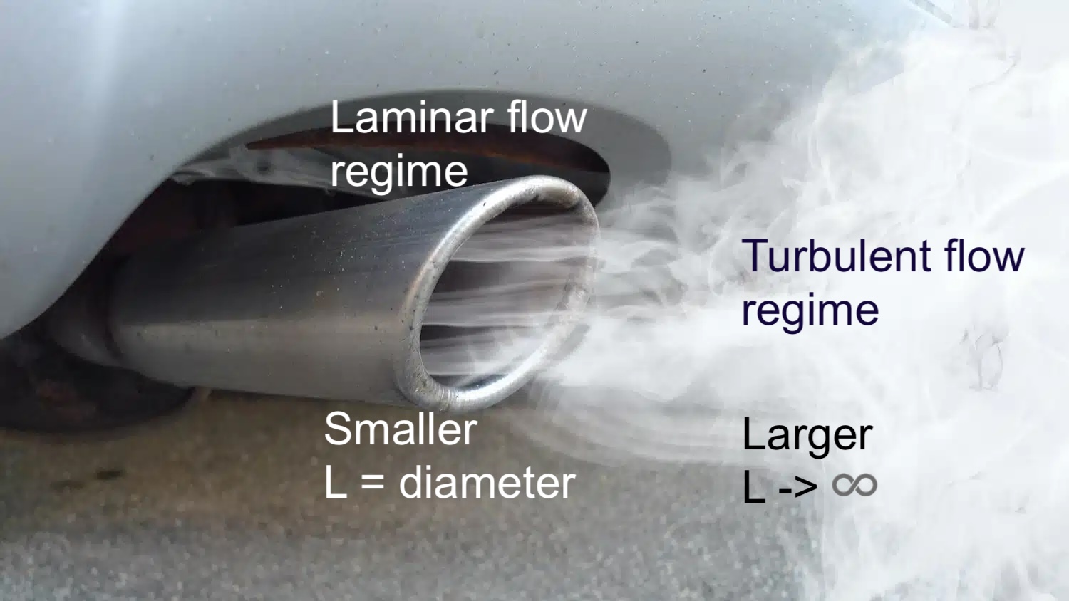
Meaning of dimensionless numbers – \(N_{Re}\)
- \(N_{Re}\): laminar flow vs turbulent flow
- Varies with characteristic length \(L_D\) (diameter for a pipe)
General procedure to calculate \(k_c'\)
Calculate Reynolds number \(N_{Re}\) from fluid properties + geometry
Determine flow regime (liquid)
- \(N_{Re} < 2100\) → laminar flow
- \(N_{Re} \ge 2100\) → turbulent flow
- Evaluate friction factor \(f\)
- Laminar flow:
\[ f = \frac{16}{N_{Re}} \] - Turbulent flow:
\[ f = \frac{\tau_s}{\tfrac12 \rho v^2},\qquad \tau_s = \frac{\Delta P_f\,\pi R^2}{2\pi R\,\Delta L} \]
Compute mass-transfer \(j\)-factor
\[ j_D = \frac{f}{2} \]Obtain mass-transfer coefficient
\[ k_c' = j_D\,v_{av}\,N_{Sc}^{-2/3} \]
Use of empirical mass transfer laws
- In many systems, flux and / or concentration profiles become hard to have simple form
- Luckily we can simplify typical mass transfer problems as different geometries
- Cyliner / Pipe
- Parallel plates
- Flow around sphere
- Packed bed
- We will show a few case studies for different geometries
- Dimensionless numbers (\(N_{Re}\), \(N_{Sc}\), \(N_{Sh}\)) help determine governing equations
Case 1: mass transfer for flow inside pipes
- Usually use the Linton & Sherwood chart
- Valid for gas / liquid in both laminar & turbulent regimes
Flow inside pipe: chart
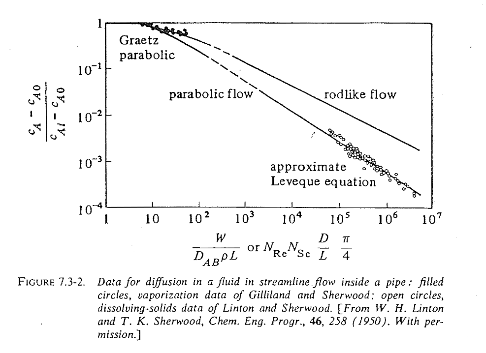
Flow inside pipes: solution procedure
- Governing dimensionless quantity:
- If gas 👉 use the “rodlike flow” line
- If liquid, distinguish 2 cases
- parabolic flow (\(N_{Re} < 2100;\ \frac{W}{D_{AB}\rho L} > 400\))
- turbulent flow (\(N_{Re} > 2100;\ 0.6 < N_{Sc} < 3000\))
Flow inside pipes: solution for liquid
Parabolic flow
\[\begin{align} \frac{c_A - c_{A,s}}{c_{A,i} - c_{A,s}} &= 5.5 \left[ \frac{W}{D_{AB}\,\rho\,L} \right]^{-\tfrac{2}{3}} \end{align}\]\(c_A\): exit concentration
\(c_{A,i}, c_{A,s}\): inlet & surface concentration
\(W\): flow rate in (kg/s)
\(k_c'\) can be calculated by \(j_D\)
Turbulent flow
\[\begin{align} N_{Sh} &= k_c'\left(\frac{D}{D_{AB}}\right) \\ &= \frac{k_c\,p_{BM}}{P} \left(\frac{D}{D_{AB}}\right) \\ &= 0.023 \left(\frac{\rho D v}{\mu}\right)^{0.83} \left(\frac{\mu}{\rho D_{AB}}\right)^{0.33} \\ &= 0.023\, N_{Re}^{0.83}\, N_{Sc}^{0.33} \end{align}\]- Similar to the \(j_D\) analog
- Just need \(N_{Re}\) and \(N_{Sc}\) to determine \(k_c'\)
- Characteristic length \(D\) is pipe diameter!
Case 2: flow past parallel plates
- Can be used for gases or evaporation of liquid
- Distinguished between laminar & turbulent flow
- \(N_{Re}\) regime cutoff different in gas & liquid!
- Characteristic length \(L\): length of plate in flow direction
Flow past parallel plates: results
Laminar flow (\(N_{Re} < 15,000\))
\[\begin{align} j_D &= 0.664 N_{Re, L}^{-0.5} \\ \frac{k_c' L}{D_{AB}} &= 0.664 N_{Re, L}^{0.5} N_{Sc}^{1/3} \end{align}\]- This follows our derivation of boundary layer theory
Turbulent flow
- Gas: \(15,000 < N_{Re}< 300,000\)
- Liquid: \(600 < N_{Re}< 50,000\)
Case 3: flow past single sphere
- Frequent geometry in particle solutions
- Low Reynolds regime 👉 solution for stagnant diffusion on spherical surface
- High Reynolds regime 👉 correct \(N_{Sh}\) and back calculate \(k_c'\)
Flow past single sphere: results
Low Reynolds (\(N_{Re} < 2\))
\[\begin{align} N_A &= \boxed{\frac{2 D_{AB}}{D_p}} (c_{A1} - c_{A2}) \\ &= k_c (c_{A1} - c_{A2}) \\ &= \frac{k_c'}{x_{Bm}}(c_{A1} - c_{A2}) \\ \end{align}\]- For \(x_{Bm} \approx 1\), we have:
\[ k_c' = \frac{2D_{AB}}{D_p} \]
- Sherwood number: \(N_{Sh} = 2\)
High Reynolds (\(N_{Re} > 2\))
- Gas:
- Liquid:
- Back calculate \(k_c' = N_{Sh} \frac{D_{AB}}{D_p}\)
Case 4: mass transfer for packed beds
- Very common geometry for chemical engineering
- Adsorption and desorption through solid particles (gases and liquids)
- Catalytic processes with very large surface area
- Geometry characteristics: void fraction \(\varepsilon\): \[
\varepsilon
= \frac{\text{void space}}{\text{total space}}
= \frac{\text{void space}}{\text{void space} + \text{solid space}}
\]
- Typically \(0.3 < \varepsilon < 0.5\)
- Void fraction is difficult to measure experimentally
Correlation equations in packed bed
Correlation 1, applicable to:
- gase with \(10 < N_{Re} <10,000\)
- liquid with \(10 < N_{Re} < 1500\)
- \(D_p\): (average) particle diameter
- \(v’\): superficial velocity in the tube without packing
Correlation equations in packed bed (II)
Correlation 2, applicable to:
- liquid with \(0.0016 < N_{Re} < 55\), \(165 < N_{Sc} < 70000\)
- liquid with \(55 < N_{Re} < 1500\), \(165 < N_{Sc} < 10690\)
Correlation equations in packed bed (III)
Correlation 3, applicable to fluidized beds
- \(10 < N_{Re} < 4000\) (gas & liquid)
- \(1 < N_{Re} < 10\) (liquid only)
Packed bed calculation steps
- Known value from operational column: \(\varepsilon\), \(V_b\) (total volume), \(D_p\), \(D_{AB}\), \(\mu\), \(\rho\), etc.
- Depend on the operational range, calculate \(N_{Re}\), \(N_Sc\) 👉 choose the equation for \(j_D\)
- Obtain \(k_c\) from \(j_D\) value
- Calculate flux \(N_A\)
- Estimate effective area \(A_{\text{eff}}\) inside the columne 👉 \(\overline{N}_A = A_{\text{eff}} N_A\)
Caveats in packed bed problems (1)
- Estimate the effective area?
- First calculate the effective surface area per volume \(a\) then \(A_{\text{eff}}\)
Caveats in packed bed problems (2)
- Use log-mean driving force (see Lecture 21)
where
- \(c_{A, i}\): surface concentration
- \(c_{A1}, c_{A2}\): in- and outlet concentrations
Caveats in packed bed problems (3)
- Mass-flow balance
where \(Q\) is the volumetric flow rate (unit m\(^3\)/s).
These equations will give rise to solving the flow in packed bed problem.
Summary
- Dimensionless numbers can be used to correlate mass transfer problems in different flow rate, dimension etc
- Typically, start with a known geometry (pipe? parallel plate? sphere? packed bed?)
- Find the correlation with dimensionless numbers \(N_{Re}\), \(N_{Sc}\)
- Calculate the final mass transfer rate