CHE 318 Lecture 22
Interface Mass Transfer
2026-03-04
Learning outcomes
After this lecture, you will be able to:
- Recall the equilibrium conditions that apply at phase interfaces.
- Describe equilibrium diagrams for two-phase mass transfer systems.
- Apply coupled flux and equilibrium relations to determine interfacial compositions.
What systems have we studies so far?
The most complex case is probably a packed-bed column.
We we have focused on?
- Mass transfer in 1 phase – gas flow over solid spheres
- Solve mass balance equation in flow direction – get outlet concentration
- Solve mass transfer to beds – get concentration profiles using fixed interfacial concentration
What we may miss?
- Real-world applications are mass transfer between 2 phases
- Mass transfer may occur across 2 phase interfaces
- Equilibrium concentration at interfaces are usually not fixed
Examples of 2-phase mass transfer (1)
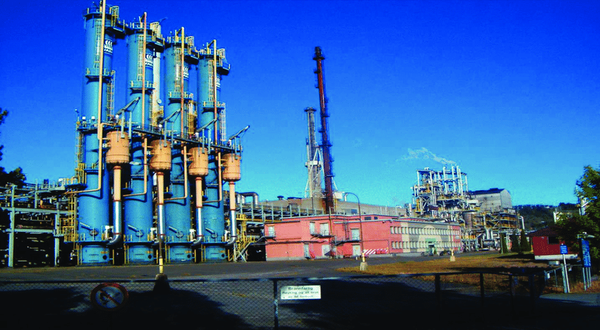
Absorption tower
- Water-soluble gases from industrial reaction mixture is transferred into aqueous solution
- Examples:
- ammonia (NH\(_3\)) from Haber-Bosch process
- CO\(_2\) capture (a hot topic!)
![]()
Examples of 2-phase mass transfer (2)
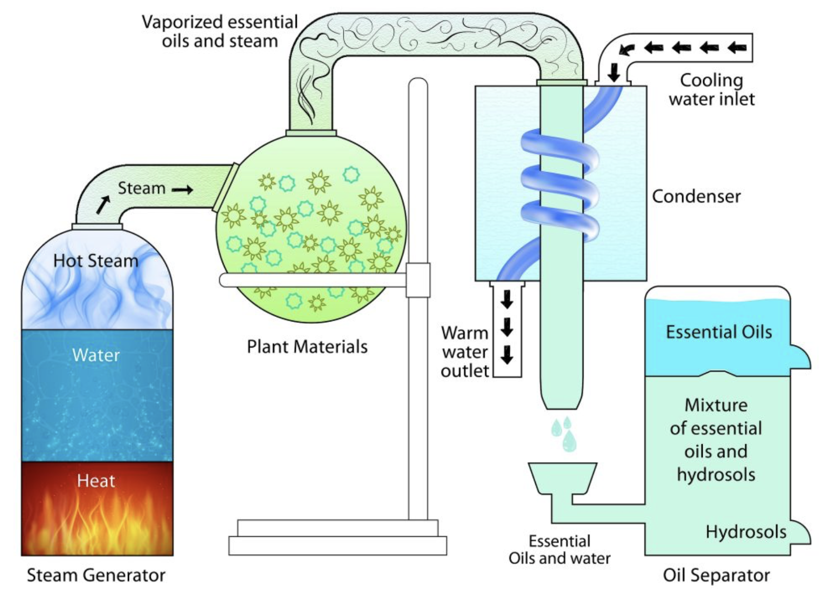
Extraction apparatus (liquid-gas)
- Volatile chemical compounds originally mixed with water are extracted to vapour phase
- Examples:
![]()
Examples of 2-phase mass transfer (3)
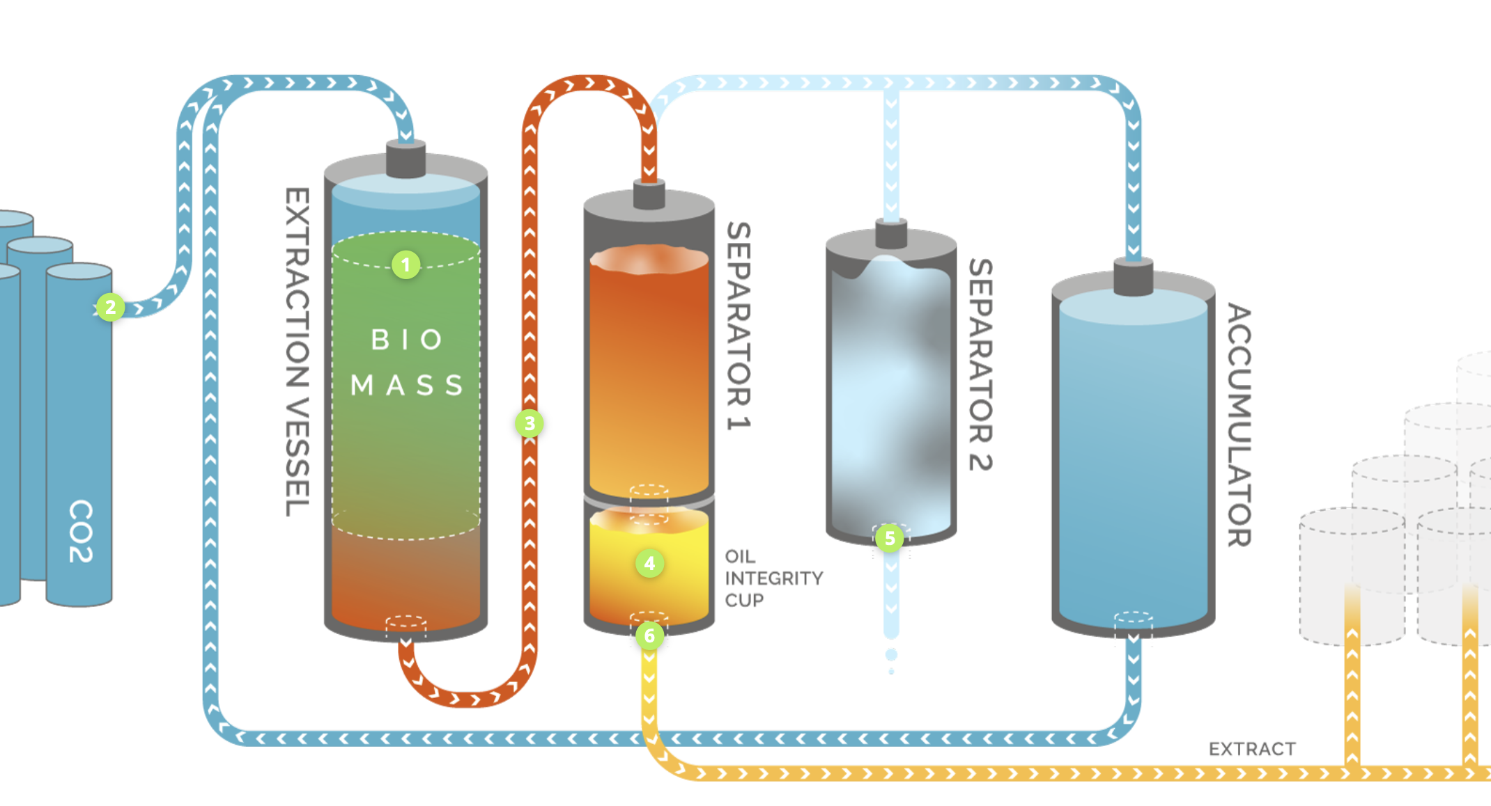
Extraction apparatus (liquid-liquid)
- Chemical compound in low solubility liquid is transferred to high solubility liquid
- Examples:
- Supercritical CO\(_2\) extraction of bioactive compounds
![]()
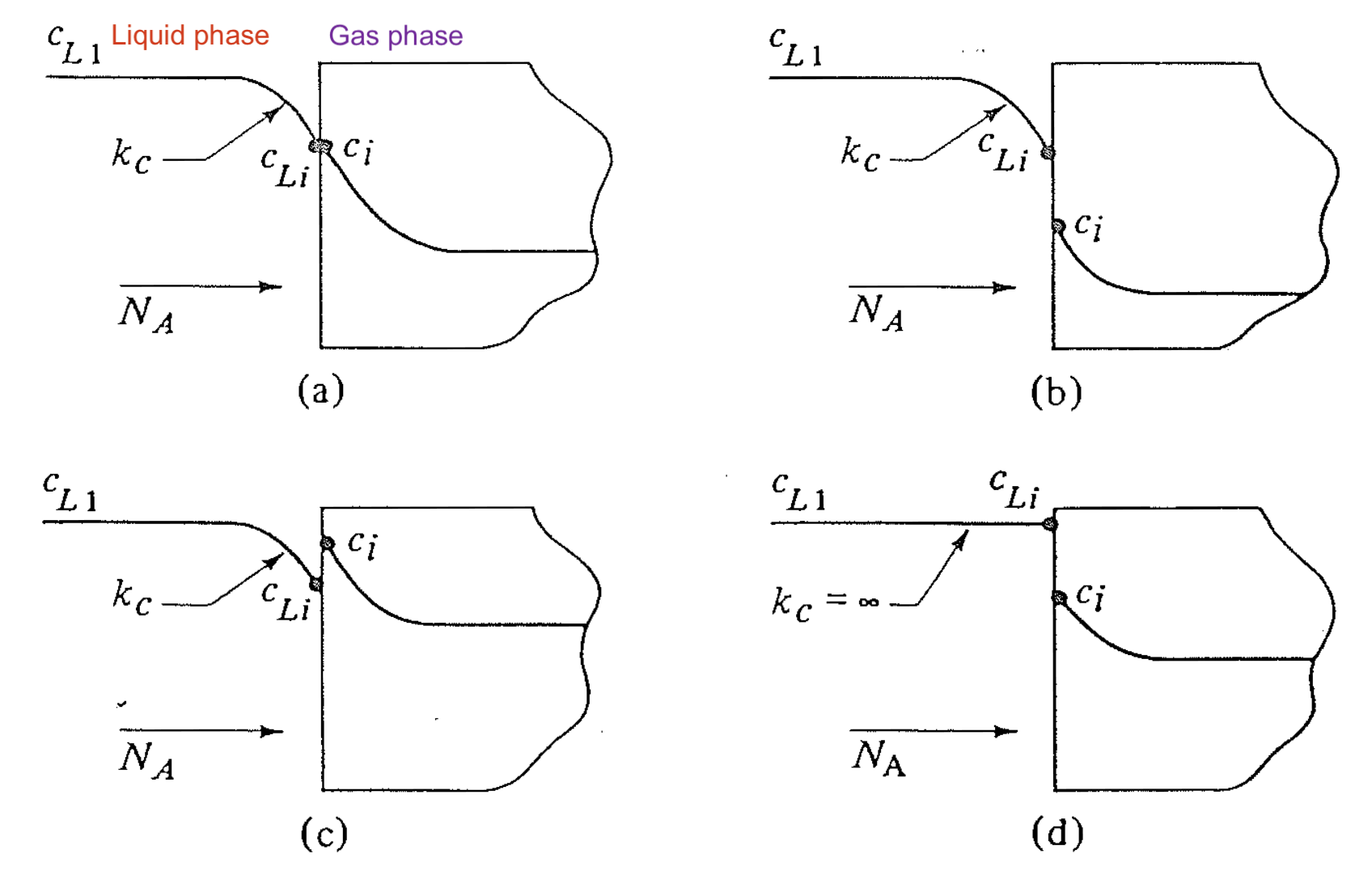
Common feature of 2-phase mass transfer
- Flow rate and interface transfer are usually orthogonal
- Interface concentration has discontinuity
![]()
Mass balance equation in 2-phase M.T.
Overall mass balance between liquid and gas
\[\begin{align}
\text{In}_{\text{liq}} + \text{In}_{\text{gas}}
=
\text{Out}_{\text{liq}} + \text{Out}_{\text{gas}}
\end{align}\]
- In and outlet usually can be described by \(\text{[Flow rate]}\times \text{[Concentration]}\)
- Depends on the direction of flow and control volume!
Mass balance equation in single phase
In each phase, we can use our knowledge from packed bed lecture, e.g.
\[\begin{align}
\text{In}_{\text{gas}} - \text{Out}_{\text{gas}} + \text{Gen}_{\text{gas}} &= 0 \\
Q (c_1 - c_2) + A_{\text{eff}} \hat{N}_{\text{eff}} &= 0
\end{align}\]
- \(\hat{N}_{\text{eff}}\) is the average molar inter-phase flux, and \(A_{\text{eff}}\) is the effective contact area
- Cannot use packed-bed solution for \(\hat{N}_{\text{eff}}\) because interfacial concentration can vary!
How can we describe the interfacial transport?
In Lecture 14 we discussed the interfacial concentration and mass balance. We need to know 1) The equilibrium constant \(K\) at the interface 2) The ratio between \(k_c'\) in two phases
![]()
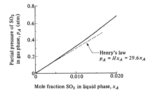
The equilibrium plot for gas-liquid interface
Most commonly in industry we can use the equilibrium plot between A’s molar fractions in gas \(y_A\) (or \(p_A\)) and liquid \(x_A\), respectively.
Simpliest situation is Henry’s law
\[
p_A = H x_A
\]
![]()
Reading an equilibrium plot (1)
Meaning of points on the equilibrium curve – interfacial concentraion
![]()
Reading an equilibrium plot (2)
- Points above the equilibrium curve 👉 \(N_A\): gas → liquid (vice versa)
![]()
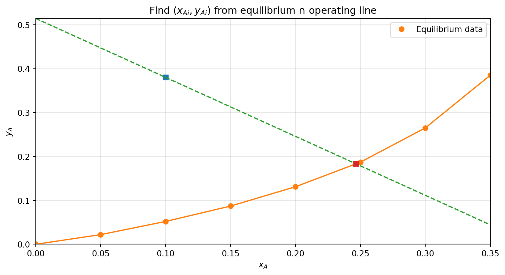
Reading an equilibrium plot (3)
- Non-equilibrium point + line with slope \(-k_x / k_y\) 👉 interfacial concentration
![]()
Equilibrium phase: flux balance
- The slope + intercept method stems from the flux balance between phases
\[\begin{align}
N_A(g) &= N_A(l) \\
k_y (y_{AG} - y_{Ai}) &= k_x (x_{Ai} - x_{AL})
\end{align}\]
\[\begin{align}
\text{Slope} &= \frac{y_{AG} - y_{Ai}}{x_{AL} - x_{Ai}} \\
&= - \frac{k_x}{k_y}
\end{align}\]
Example 1: solution plot
Interface concentrations: x_Ai = 0.246589, y_Ai = 0.183180
N_A from gas film:    2.883412e-04 (same units as k_y)
N_A from liquid film: 2.883412e-04 (same units as k_x)
Example 1: answers
- Slope of curve \(-k_x/k_y = -1.343\)
- Interfacial concentration \((x_{Ai}, y_{Ai}) = (0.246, 0.180)\)
- Flux: \(N_A =0.29 \times 10^{-3}\) kg mol/m\(^2\)/s
- Direction of flux: gas to liquid
Summary
- Real industrial applications involve mass transfer between 2 phases
- Equilibrium plots are extremely useful for elucidating the interfacial balance
- Describe driving force and interfacial concentrations from the equilibrium plot