---
title: "CHE 318 Lecture 22"
subtitle: "Interface Mass Transfer"
author: "Dr. Tian Tian"
date: "2026-03-04"
format:
html: {}
revealjs:
output-file: slides.html
pdf:
output-file: L22.pdf
---
::: {.content-visible when-format="html" unless-format="revealjs"}
::: {.callout-note}
- Slides 👉 [Open presentation🗒️](./slides.html)
- PDF version of course note 👉 [Open in pdf](./L22.pdf)
- Handwritten notes 👉 [Open in pdf](./public/L22_annotated.pdf)
:::
:::
## Learning outcomes {.center}
After this lecture, you will be able to:
- **Recall** the equilibrium conditions that apply at phase interfaces.
- **Describe** equilibrium diagrams for two-phase mass transfer systems.
- **Apply** coupled flux and equilibrium relations to determine interfacial compositions.
## What systems have we studies so far?
The most complex case is probably a packed-bed column.
- We we have focused on?
- Mass transfer in **1 phase** -- gas flow over solid spheres
- Solve mass balance equation in flow direction -- get **outlet** concentration
- Solve mass transfer to beds -- get concentration profiles using **fixed interfacial concentration**
- What we may miss?
- Real-world applications are mass transfer between 2 phases
- Mass transfer may occur across 2 phase interfaces
- Equilibrium concentration at interfaces are usually not fixed
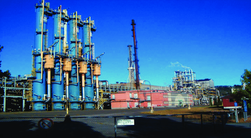
## Examples of 2-phase mass transfer (1)
**Absorption tower**
- Water-soluble gases from industrial reaction mixture is transferred into aqueous solution
- Examples:
- ammonia (NH$_3$) from Haber-Bosch process
- CO$_2$ capture (a hot topic!)
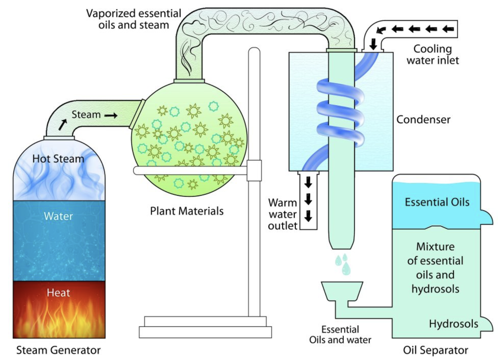
## Examples of 2-phase mass transfer (2)
**Extraction apparatus** (liquid-gas)
- Volatile chemical compounds originally mixed with water are extracted to vapour phase
- Examples:
- Essence oil extraction
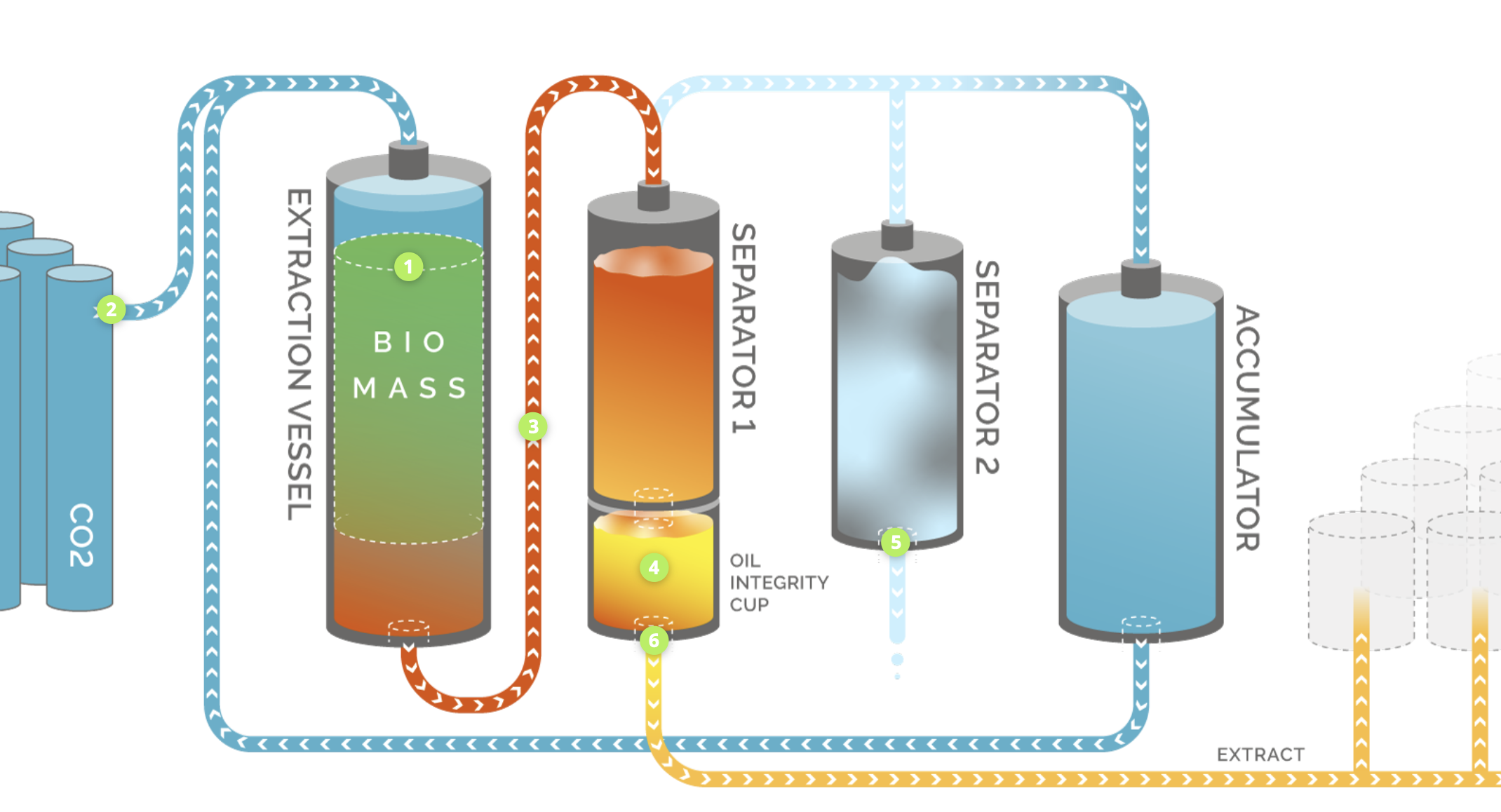
## Examples of 2-phase mass transfer (3)
**Extraction apparatus** (liquid-liquid)
- Chemical compound in low solubility liquid is transferred to high solubility liquid
- Examples:
- Supercritical CO$_2$ extraction of bioactive compounds
## Common feature of 2-phase mass transfer
- Flow rate and interface transfer are usually orthogonal
- Interface concentration has discontinuity

## Mass balance equation in 2-phase M.T.
Overall mass balance between liquid and gas
```{=tex}
\begin{align}
\text{In}_{\text{liq}} + \text{In}_{\text{gas}}
=
\text{Out}_{\text{liq}} + \text{Out}_{\text{gas}}
\end{align}
```
- In and outlet usually can be described by $\text{[Flow rate]}\times \text{[Concentration]}$
- Depends on the direction of flow and control volume!
## Mass balance equation in single phase
In each phase, we can use our knowledge from [packed bed lecture](../L21), e.g.
```{=tex}
\begin{align}
\text{In}_{\text{gas}} - \text{Out}_{\text{gas}} + \text{Gen}_{\text{gas}} &= 0 \\
Q (c_1 - c_2) + A_{\text{eff}} \hat{N}_{\text{eff}} &= 0
\end{align}
```
- $\hat{N}_{\text{eff}}$ is the average molar inter-phase flux, and $A_{\text{eff}}$ is the effective contact area
- Cannot use packed-bed solution for $\hat{N}_{\text{eff}}$ because interfacial concentration can vary!
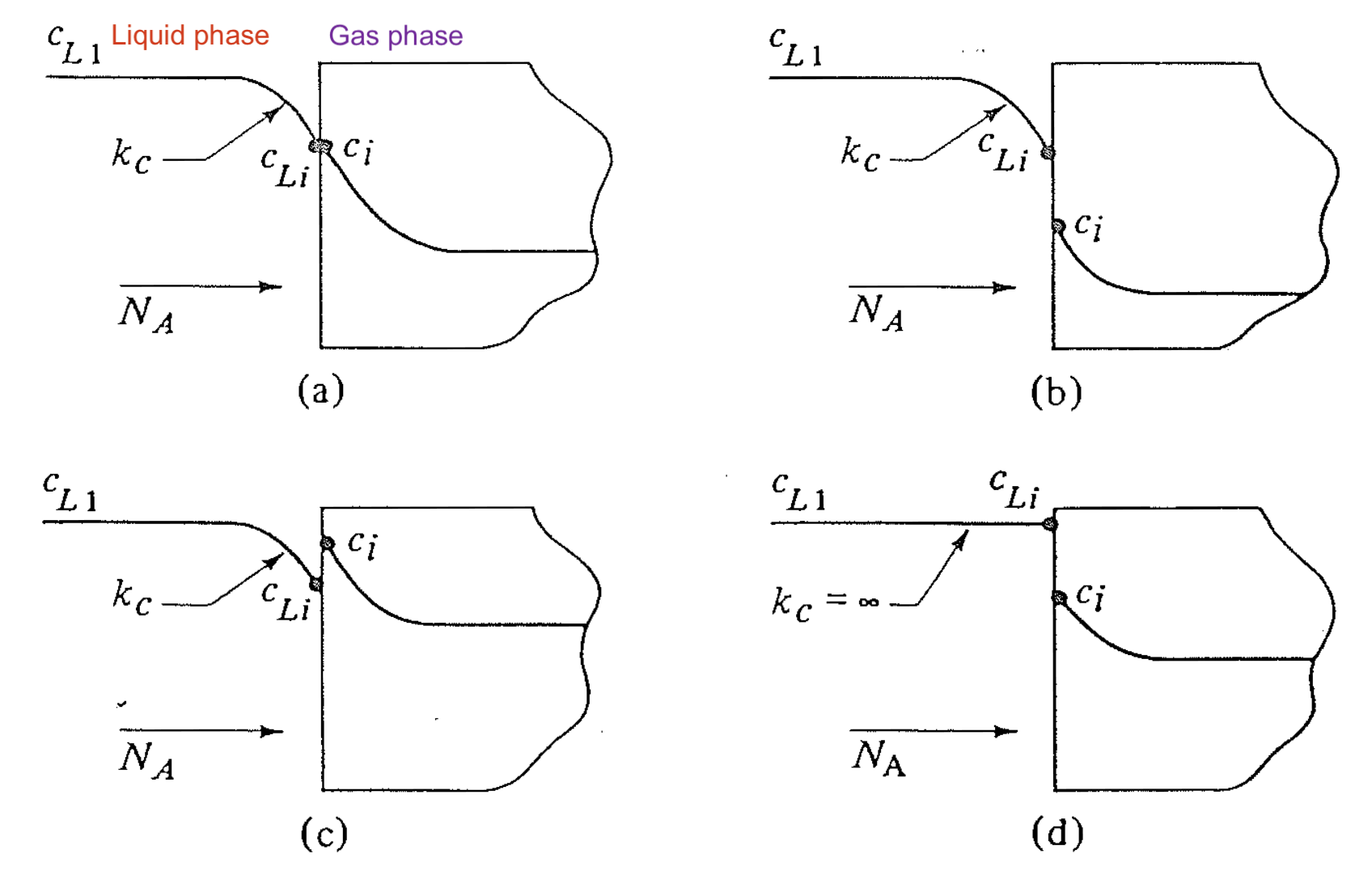
## How can we describe the interfacial transport?
In [Lecture 14](../L14) we discussed the interfacial concentration and mass balance. We need to know
1) The equilibrium constant $K$ at the interface
2) The ratio between $k_c'$ in two phases
{width="95%"}
## The equilibrium plot for gas-liquid interface
Most commonly in industry we can use the equilibrium plot between A's
molar fractions in gas $y_A$ (or $p_A$) and liquid $x_A$, respectively.
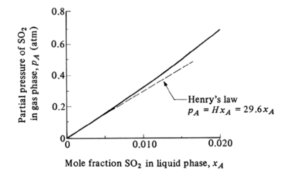
Simpliest situation is Henry's law
$$
p_A = H x_A
$$
## Reading an equilibrium plot (1)
Meaning of points on the equilibrium curve -- interfacial concentraion

## Reading an equilibrium plot (2)
- Points above the equilibrium curve 👉 $N_A$: gas → liquid (vice versa)

## Reading an equilibrium plot (3)
- Non-equilibrium point + line with slope $-k_x / k_y$ 👉 interfacial concentration

## Equilibrium phase: flux balance
- The slope + intercept method stems from the flux balance between phases
```{=tex}
\begin{align}
N_A(g) &= N_A(l) \\
k_y (y_{AG} - y_{Ai}) &= k_x (x_{Ai} - x_{AL})
\end{align}
```
- We have
```{=tex}
\begin{align}
\text{Slope} &= \frac{y_{AG} - y_{Ai}}{x_{AL} - x_{Ai}} \\
&= - \frac{k_x}{k_y}
\end{align}
```
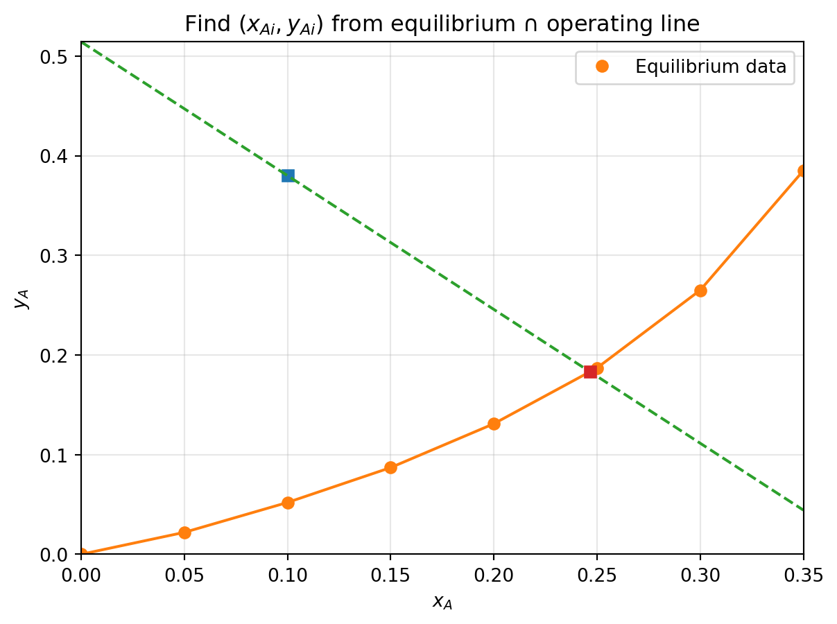
## Example 1: finding equilibrium interface concentrations
A solute is being absorbed from a gas mixture of A and B in a
wetted-wall tower, with the liquid flowing downwards. At a certain
point in the tower, the bulk gas concentration of A is $y_{AG}=0.380$
and the bulk liquid fraction is $x_{AL}=0.100$. The film transfer
coefficients for A in gas and liquid phases are: $k_y'=1.465\times 10^{-3}$ kg mol/m$^2$/s and $k_x'=1.967\times 10^{-3}$ kg mol/m$^2$/s. You can assume the $k_x' \approx k_x$ and $k_y' \approx k_y$. The following pairs of equilibrium $(x_Ai, y_Ai)$ data were measured:
$(0.0, 0.0), (0.05, 0.022), (0.10, 0.052) (0.15, 0.087)$
$(0.20, 0.131), (0.25, 0.187), (0.30, 0.265), (0.35, 0.385)$
1) Find the interface concentrations $y_{Ai}$ and $x_{Ai}$
2) Calculate the $N_A$ at this point
## Solution steps:
1) Draw the equilbirum plot with interpolation
2) Draw the current $(x_{AL}, y_{AG})$ point on graph, which direction of mass transfer?
3) Draw line with slow of $-k_x/k_y$
4) Read the intersect with equilibrium curve as $(x_{Ai}, y_{Ai})$
5) Calculate $N_A = k_y (y_{AG} - y_{Ai})$
## Example 1: solution plot
```{python}
#| echo: false
import numpy as np
import matplotlib.pyplot as plt
# Given bulk compositions
y_AG = 0.380
x_AL = 0.100
# Given film coefficients (treat as ky, kx per problem statement)
k_y = 1.465e-3
k_x = 1.967e-3
# Equilibrium data (x_Ai, y_Ai)
x_eq = np.array([0.0, 0.05, 0.10, 0.15, 0.20, 0.25, 0.30, 0.35])
y_eq = np.array([0.0, 0.022, 0.052, 0.087, 0.131, 0.187, 0.265, 0.385])
# Operating line from two-film theory:
# N_A = k_y (y_AG - y_i) = k_x (x_i - x_AL)
# => y_i = y_AG - (k_x/k_y) (x_i - x_AL)
m = -(k_x / k_y)
b = y_AG - m * x_AL # y = m x + b
def y_oper(x):
return m * x + b
# Piecewise-linear interpolation of equilibrium curve and intersection with operating line
# Find interval where (y_eq - y_oper(x_eq)) changes sign
g = y_eq - y_oper(x_eq)
idx = np.where(np.sign(g[:-1]) * np.sign(g[1:]) <= 0)[0]
if len(idx) == 0:
raise RuntimeError("No intersection found within provided equilibrium data range.")
i = idx[0]
# Linear interpolation on [x_i, x_{i+1}] for equilibrium: y = y0 + (y1-y0)*(x-x0)/(x1-x0)
x0, x1 = x_eq[i], x_eq[i+1]
y0, y1 = y_eq[i], y_eq[i+1]
s = (y1 - y0) / (x1 - x0) # equilibrium segment slope
# Solve y_eq_lin(x) = y_oper(x):
# y0 + s (x - x0) = m x + b
x_int = (y0 - s * x0 - b) / (m - s)
y_int = y_oper(x_int)
# Flux at the point
N_A_gas = k_y * (y_AG - y_int)
N_A_liq = k_x * (x_int - x_AL)
print(f"Interface concentrations: x_Ai = {x_int:.6f}, y_Ai = {y_int:.6f}")
print(f"N_A from gas film: {N_A_gas:.6e} (same units as k_y)")
print(f"N_A from liquid film: {N_A_liq:.6e} (same units as k_x)")
# Plot
xx = np.linspace(x_eq.min(), x_eq.max(), 400)
plt.figure()
plt.plot(0.100, 0.380, "s")
l, = plt.plot(x_eq, y_eq, "o", label="Equilibrium data")
plt.plot(xx, np.interp(xx, x_eq, y_eq), "-", color=l.get_c())
plt.plot(xx, y_oper(xx), "--",)
plt.plot([x_int], [y_int], "s")
plt.xlabel(r"$x_A$")
plt.ylabel(r"$y_A$")
plt.title(r"Find $(x_{Ai}, y_{Ai})$ from equilibrium ∩ operating line")
plt.xlim(x_eq.min(), x_eq.max())
plt.ylim(min(0, y_oper(x_eq).min(), y_eq.min()), max(y_oper(x_eq).max(), y_eq.max()))
plt.grid(True, alpha=0.3)
plt.legend()
plt.show()
```
## Example 1: answers
- Slope of curve $-k_x/k_y = -1.343$
- Interfacial concentration $(x_{Ai}, y_{Ai}) = (0.246, 0.180)$
- Flux: $N_A =0.29 \times 10^{-3}$ kg mol/m$^2$/s
- Direction of flux: gas to liquid
## Summary
- Real industrial applications involve mass transfer between 2 phases
- Equilibrium plots are extremely useful for elucidating the interfacial balance
- Describe driving force and interfacial concentrations from the equilibrium plot