MATE 664 Lecture 19
Colloidal Stability: DLVO Theory
2026-03-16
Learning outcomes
After this lecture, you will be able to:
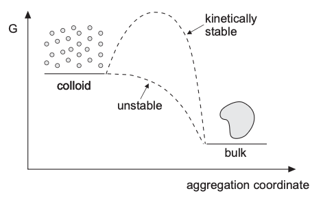
- Explain why a thermodynamically unstable colloid may still remain dispersed
- Describe the physical origin of van der Waals attraction and double-layer repulsion
- Use the Poisson-Boltzmann equation and its boundary conditions for a charged interface
- Recall the Debye length and the role of ionic strength
- State the DLVO interaction potential and interpret the barrier height
- Connect DLVO theory to the RLCA picture from last lecture
Recap: why did RLCA become slow?
Last lecture, we introduced a kinetic barrier through the external potential \(V_T\):
\[\begin{align} F = 4\pi r^2 D_{11} \left( \frac{dN}{dr} + \frac{N}{k_B T}\frac{dV_T}{dr} \right) \end{align}\]and the Fuchs stability ratio
\[\begin{align} W = \frac{\beta_{11}^{\mathrm{DLCA}}}{\beta_{11}^{\mathrm{RLCA}}} \end{align}\]The missing question
When we introduce the external potential \(V_T\) (and \(W\)) we show the RLCA rate is slower, but why?
- what determines \(V_T(r)\)?
- why does a barrier appear?
- how can salt destroy the barrier?
Today: physical origin of kinetic stability
Derjaguin, Landau, Verwey, and Overbeek (DLVO) theory: For charged colloids, the total interaction potential comes from two competing effects:
- attractive van der Waals interaction
- repulsive electrostatic double-layer interaction
DLVO theory combines them into one total potential.
\[\begin{align} V_T(h) = V_{\mathrm{vdW}}(h) + V_{\mathrm{el}}(h) \end{align}\]
where \(h\) is the surface-to-surface separation.
Stability statement revisited
From Lecture 18, a lyophobic colloid remains only metastable. The dispersed state has higher free energy than the aggregated state, but aggregation may be delayed if particles must overcome a barrier.
Key idea:
- thermodynamics favors aggregation
- kinetics may prevent close contact
- barrier height should be compared with \(k_B T\)
What should the DLVO curve look like?
A typical interaction curve contains (how do they come)?
- a deep primary minimum at very short range
- a repulsive maximum at intermediate separation
- sometimes a shallow secondary minimum at larger separation

Topic 1: electrostatic double layer around a charged particle
A charged solid surface in electrolyte attracts counterions and repels coions. This creates the electrical double layer:

Electrostatic potential from Poisson equation
The potential field \(\psi\) in a dielectric medium satisfies Poisson equation (one of Maxwell’s equations)
- \(\rho\): local charge density
- \(\varepsilon_r \varepsilon_0\): permittivity of the liquid

Ion distribution from Boltzmann statistics
For ion species \(i\) with valence \(z_i\), the equilibrium concentration follows
\[\begin{align} n_i = n_{i,\infty} \exp \left( -\frac{z_i e \psi}{k_B T} \right) \end{align}\]Hence the charge density \(\rho\) in Poisson equation is
\[\begin{align} \rho = \sum_i z_i e n_i = \sum_i z_i e n_{i,\infty} \exp \left( -\frac{z_i e \psi}{k_B T} \right) \end{align}\]Linking this to the Poisson equation gives the Poisson-Boltzmann (PB) equation
Poisson-Boltzmann equation
Combining Poisson and Boltzmann gives the nonlinear PB equation
\[\begin{align} \nabla^2 \psi = -\frac{1}{\varepsilon_r \varepsilon_0} \sum_i z_i e n_{i,\infty} \exp \left( -\frac{z_i e \psi}{k_B T} \right) \end{align}\]For a symmetric electrolyte and planar geometry, this becomes the standard 1D form.
Solution to the PB equation: planar geometry and boundary conditions
Take \(x\) normal to a flat charged surface. Far from the surface, the solution must recover bulk electroneutrality:
\[\begin{align} \psi(x \rightarrow \infty) &= 0 \\ \frac{d\psi}{dx}(x \rightarrow \infty) &= 0 \end{align}\]At the surface, two common boundary conditions are used.
Boundary condition 1: constant surface potential
If the surface potential can be predetermined (like zeta-potential measurements), then
\[\begin{align} \psi(0) = \psi_0 \end{align}\]This is often used when adsorption or surface chemistry keeps the interfacial potential nearly fixed.
Boundary condition 2: constant surface charge
Using Gauss law, the electric field at the surface satisfies
\[\begin{align} \sigma = -\varepsilon_r \varepsilon_0 \frac{d\psi}{dx}\Big|_{x=0} \end{align}\]This is the constant-charge description, applicable to:
- more natural if surface groups are fixed (e.g. chemically modified)
- important when particle approach changes the local field
Solution to Poisson-Boltzmann: Debye-Hückel linearization
If the potential is not too large,
\[\begin{align} \left| \frac{z_i e \psi}{k_B T} \right| \ll 1 \end{align}\]then the PB equation can be linearized, often called the Debye-Hückel (DH) approximation
\[\begin{align} \exp \left( -\frac{z_i e \psi}{k_B T} \right) \approx 1 - \frac{z_i e \psi}{k_B T} \end{align}\]Potential profile in Debye-Hückel approximation
The linearized equation in DH approximation becomes
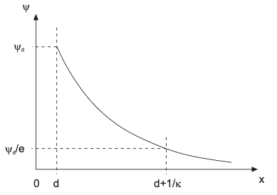
\[\begin{align} \frac{d^2 \psi}{dx^2} = \kappa^2 \psi \end{align}\]We know from the diffusion concepts it is like a steady-state Fick’s second law, but with external potential. The solution is a nice exponential decay of potential \(\psi\)
\[\begin{align} \psi(x) = \psi_0 e^{-\kappa x} \end{align}\]Debye-Hückel approximation: screening length
One consequence of the DH approximation is that the electrostatic screening is related with the charge concentrations in the liquid:
\[\begin{align} \kappa^{-1} &= \left( \frac{\varepsilon_r \varepsilon_0 k_B T} {e^2 \sum n_{i, 0} z_i^2} \right)^{1/2} \\ &= \left( \frac{\varepsilon_r \varepsilon_0 k_B T} {2 e^2 N_a I} \right)^{1/2} \end{align}\]where \(N_a\) is the Avogadro number, and \(I = 1/2 \sum_{i} z_{i}^{2} c_{i, 0}\) is the ionic strength.
- high ionic strength \(I\) \(\rightarrow\) shorter screening length
- low ionic strength \(I\) \(\rightarrow\) longer-range repulsion
In-depth view of the screening length
From the Debye-Hückel Approximation, we typically can use the following handy rule:
\[ \kappa = 3.29 \sqrt{I} = 3.29 \sqrt{\frac{1}{2}\sum c_{i, 0} z_i^2}\qquad \text{[nm]}^{-1} \]
when the solute concentration \(c_{i, 0}\) is in mol/L. For example, for a \(10^{−3}\) M, 1:1 electrolyte, \(1/\kappa = 9.6\) nm.
Shape of Debye-Hückel approximation
Where can I find the screening length \(\kappa^{-1}\)?
Poisson-Boltzmann in high potential regime: Guy-Chapman equation
The Debye–Hückel approximation assumes small potential
\[\begin{align} \left|\frac{ze\psi}{k_B T}\right| \ll 1 \end{align}\]For a higher surface potential, the Gouy-Chapman (GC) equation is more accurate (exact solution for symmetric electrolyte.
\[\begin{align} \frac{d^{2} \psi}{dx^{2}} &= -\frac{zc_{0}e}{\varepsilon_{o} \varepsilon_{r}} \left[ \exp(-\frac{ze\psi}{k_{\mathrm{B}}T}) - \exp(\frac{ze\psi}{k_{\mathrm{B}}T})\right]\\ &= \frac{2zc_{0}e}{\varepsilon_{o} \varepsilon_{r}} \sinh\left(\frac{ze\psi}{k_{\mathrm{B}}T}\right) \end{align}\]Solution to the GC equation is:
\[ \frac{\tanh(ze\psi/4k_{\mathrm{B}}T)}{\tanh(ze\psi_{0}/4k_{\mathrm{B}}T)} = \exp(-\kappa x) \]
Repulsion between two charged plates
When two charged surfaces approach, their diffuse layers overlap. You can imagine the charge-redistribution occurs between the two surfaces. Let’s first assume the charged surfaces are flat surfaces, the overlay will cause osmotic pressure.

The osmotic pressure
In an ideal electrolyte solution, the local osmotic pressure follows the Donnan equation
\[ P_{\mathrm{osmotic}}(x) = k_B T \left(c_{+}(x) + c_{-}(x)\right) \]
Force balance inside the double layer
Consider a differential volume element \(dV\) located at position \(x\).
The differential osmotic force acting on the element is
\[\begin{align} dF_{\mathrm{osmotic}} = \frac{dP_{\mathrm{osmotic}}}{dx} dV \end{align}\]Solving the parallel charge plate: osmotic pressure
The equilibrium requires the electrostatic force and osmotic force must balance at every position.
\[\begin{align} \frac{dP_{\mathrm{osmotic}}}{dx} &= \varepsilon_0\varepsilon_r \frac{d^2\psi}{dx^2} \frac{d\psi}{dx} \\ &= \frac{\varepsilon_0\varepsilon_r}{2} \frac{d}{dx} \left[ \left(\frac{d\psi}{dx}\right)^2 \right] \end{align}\]Since we know the solution to the Poisson-Boltzmann equation, integrating this will give us the total interaction energy.
Repulsion between charged planes: final result
The repulsive potential energy \(W_{\mathrm{R}}\) per unit area between two charged particles at distance \(h\) is then calculated as:
\[\begin{align} W_{\mathrm{R}}(h) &= -\int_{\infty}^{h} \frac{F_{\mathrm{R}}}{A} \mathrm{d} h' \\ &= 64 k T c_{0} \kappa^{-1} \Lambda_{0}^{2} e^{-\kappa h} \end{align}\]where \(\Lambda_{0} = \tanh(\frac{z e \psi_{0}}{4k_{\mathrm{B}}T})\). Note we need to adjust for the particle curvature if they are spheres.
Why do we care about curvature?
The plate result is not yet the particle result. Real colloids are spherical, so we must convert planar interaction into curved-particle interaction. Derjaguin approximation calculates the electrostatic repulsion between sphere particles by:
\[\begin{align} V(h) = 2\pi R_{\mathrm{eff}} W(h) \end{align}\]where \(W(h)\) is the interaction free energy per unit area between plates. This is our final solution
Effective curvature radius
For two particles of radii \(a_1\) and \(a_2\),
\[\begin{align} R_{\mathrm{eff}} = \frac{a_1 a_2}{a_1+a_2} \end{align}\]For equal particles, \(a_1=a_2=a\):
\[\begin{align} R_{\mathrm{eff}} = \frac{a}{2} \end{align}\]- large particles have stronger total interaction
- curvature links plate theory to colloid kinetics
Topic 1: final form
The repulsion between two spherical particles separated by \(h\) under the Derjarguin approximation is
\[ V_{\mathrm{R}}^{\mathrm{ss}}(h) = 64 \pi k_B T c_{0} R \kappa^{-2} \Lambda_{0}^{2} e^{-\kappa h} \]
Such approximation is valid when:
- \(R \gg h\), i.e. near the junction the surfaces from two particles are still considered as planar.
- \(h \gg \kappa^{-1}\), i.e. small overlap between EDLs.
Topic 2: van der Waals attraction
The attractive branch comes from fluctuating dipoles. At the molecular level, we have interaction between two particles following the \(r^{-6}\) rule
\[\begin{align} u(r) = -\frac{C}{r^6} \end{align}\]Summing over all pair interactions between two bodies gives the macroscopic van der Waals interaction. The material dependence is collected into the Hamaker constant \(A_H\).
Simple van der Waals result for curved particles
For two spheres at small separation \(h \ll a_1, a_2\),
\[\begin{align} V_{\mathrm{vdW}}(h) = -\frac{A_H R_{\mathrm{eff}}}{6h} \end{align}\]For equal particles with radius \(a\),
\[\begin{align} V_{\mathrm{vdW}}(h) = -\frac{A_H a}{12h} \end{align}\]- attraction becomes very strong at small \(h\)
- this is the origin of the primary minimum
DLVO total interaction potential
Putting both parts from repulsive electrostatics and attractive vdW together gives the central DLVO expression:
\[\begin{align} V_T(h) = -\frac{A_H R_{\mathrm{eff}}}{6h} + B R_{\mathrm{eff}} e^{-\kappa h} \end{align}\]DLVO kinetic barrier
This single curve explains both stabilization and aggregation.
Barrier criterion for kinetic stability
The key quantity is the maximum barrier height \(V_{T,\max}\) in the DLVO curve.
- Stable regime
particle collisions usually do not lead to sticking.
- Unstable regime
then particles can cross the barrier and aggregate.
This is the physical origin of RLCA.
Salt effect and critical coagulation concentration
Increasing salt compresses the double layer:
\[\begin{align} \kappa \propto I^{1/2} \end{align}\]Consequences:
- repulsion becomes shorter-ranged
- barrier height decreases
- aggregation rate increases
At a sufficiently high salt level, the barrier vanishes. This defines the critical coagulation concentration.
DLVO theory in the language of last lecture
In Lecture 18 we wrote
\[\begin{align} \beta_{11}^{\mathrm{RLCA}} = \frac{\beta_{11}^{\mathrm{DLCA}}}{W} \end{align}\]and
\[\begin{align} W \approx \frac{1}{2\kappa a} \exp \left( \frac{V_{T,\max}}{k_B T} \right) \end{align}\]Now we can interpret this clearly:
- DLVO gives the potential \(V_T(h)\)
- the barrier maximum controls \(W\)
- \(W\) then controls the slowdown from DLCA to RLCA
What DLVO theory captures well
- electrostatic stabilization of lyophobic colloids
- salt-induced destabilization
- barrier-controlled transition from stable to aggregating
- connection between interparticle forces and kinetic rate constants
It is the simplest quantitative framework for charged colloidal stability.
What is not included in simple DLVO?
DLVO is powerful, but not complete. Missing effects include:
- steric stabilization by adsorbed polymers
- hydration forces at very short range
- charge regulation during particle approach
- non-spherical rough particles
- specific ion effects
These extensions are often needed in real polymer and ceramic systems.
Summary
- A colloid may be thermodynamically unstable but kinetically stable
- DLVO theory combines attraction and repulsion
- van der Waals attraction scales roughly as \(-1/D\)
- double-layer repulsion decays as \(e^{-\kappa D}\)
- the barrier height relative to \(k_B T\) determines whether aggregation is DLCA-like or RLCA-like
- increasing salt lowers the barrier and promotes coagulation