CHE 318 Lecture 04
Molecular Diffusivity: Theories and Measurement
2026-01-12
Note
Recap
- General solution for diffusion binary mixture gas systems (\(N_B = k N_A\))
- \(k = -1\) reduces to EMCD solution
- Total flux \(N_A\) is EMCD flux times a coefficient
- Brief discussion about diffusivity measurement: two-bulb setup
Demonstration of general solution
Interaction time!
Results and comments to be published after the class
Convection-driven flux change

Figure 1
Learning outcomes
After this lecture, you will be able to:
- Recall major theories used to estimate molecular diffusivity.
- Describe how the diffusivity \(D_{AB}\) changes with temperature and pressure.
- Apply tabulated reference data to estimate diffusivity values.
- Formulate governing equations for common diffusivity-measurement scenarios.
Let’s look at the general mass transfer equation (again)
\[ N_A = \frac{D_{AB} c_T}{(z_2 - z_1)} s \ln\!\left[\dfrac{ s - \frac{c_{A2}}{c_T}} {s - \frac{c_{A1}}{c_T}} \right] \quad s = \frac{N_A}{N_A + N_B} \]
What values do we know from the system setup?
- Geometry: \(z_1\), \(z_2\), \(c_{A1}\), \(c_{A2}\), \(c_T\)
- Chemical reaction stoichiometry: \(k\)
What else value(s) do we need to solve \(N_A\)?
- \(D_{AB}\): generally \(D_{AB}(z) = \text{Const}\)
- But \(D_{AB}=f(T, P, \cdots)\)
Motivation to have theory about diffusivity
- Solving the general solution for gas mass transfer requires parameter \(D_{AB}\) (and \(D_{BA}\))!
- Measuring every \(D_{AB}\) pair for gases is tedious
- \(D_{AB}\) is dependent on conditions \(T, P\)
- We need to have theories that can predict diffusivity \(D_{AB}\) without doing all pair experiments and all \((T, P)\) conditions!
- In the lease case, the theory should allow extrapolating a measured \(D_{AB}(T_1, P_1)\) to \(D_{AB}(T_2, P_2)\)
Molecular diffusivity theory – kinetic theory
In dilute gas regime (\(p_T \approx \text{atm}\)), the kinetic behaviour of gas molecules can be described using kinetic theory. A few assumptions are made:
- Interdiffusion between A and B are dominated by collision between molecules (low \(p_T\) 👉 only 2 molecules can collide at the same time)
- The molecules are rigid spheres having particle masses \(m_A\), \(m_B\) and diameters \(d_A\) and \(d_B\)
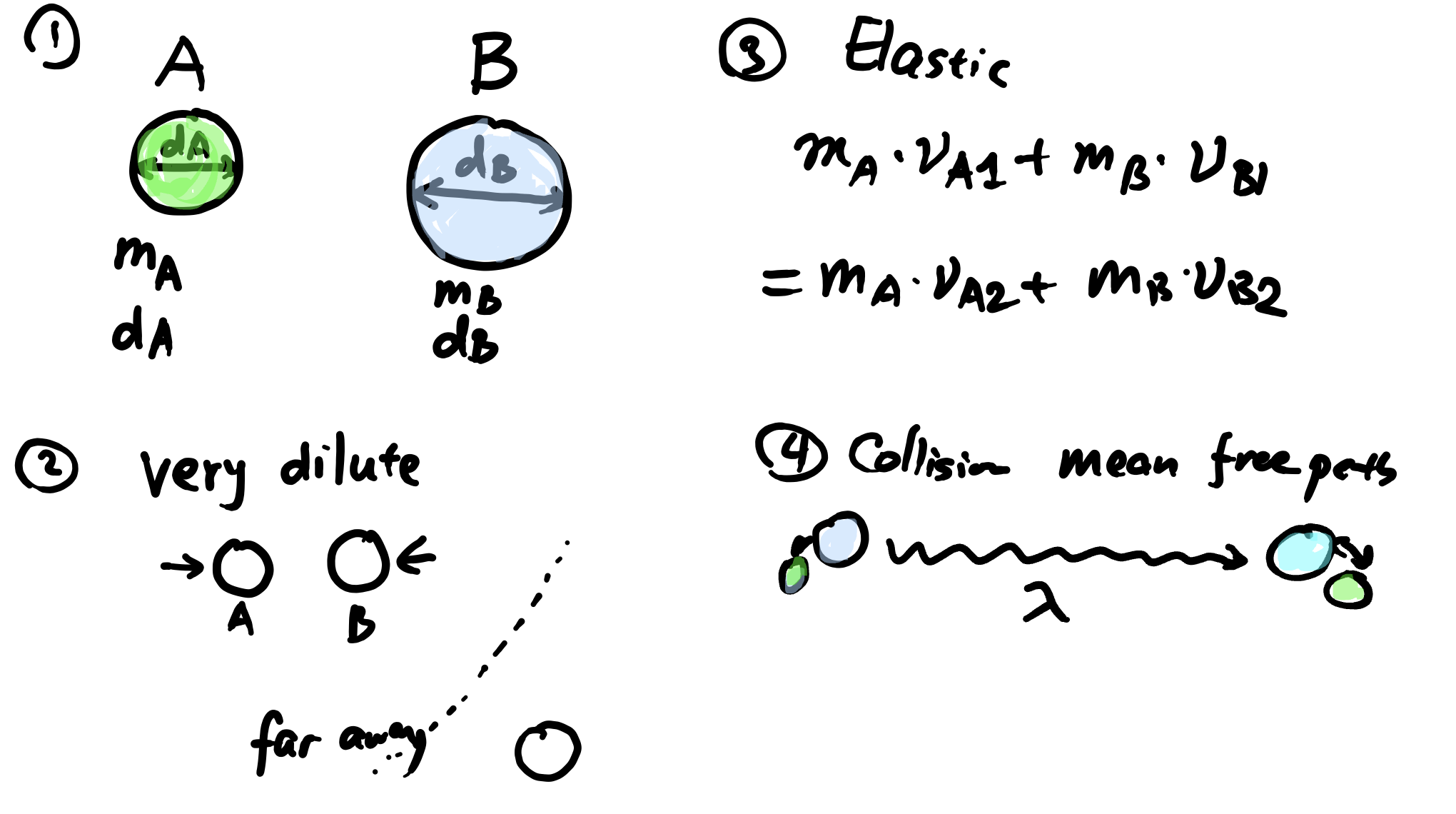
Scheme of gas kinetic theory
Kinetic theory – key results
There are some results from the kinetic theory: 1
Mean molecular speed \(\overline{u}\) \[ \overline{u} = \sqrt{\frac{8 k_B T}{\pi \overline{m_{AB}}}} \]
Mean free path (between collisions): \(\lambda_{A,B}\) \[ \lambda_{AB}=\frac{1}{\sqrt{2} \pi d_{AB}^2 c_T} \]
- Frequency of molecule A colliding with wall (\(Z\), unit \(\text{m}^{-2}\cdot \text{s}^{-1}\)): \[ Z_A = \frac{1}{4} c_A \overline{u} \]
where \(d_{AB} = \frac{d_A + d_B}{2}\), \(m_{AB}^{-1} = m_{A}^{-1} + m_B^{-1}\), \(k_B\) is the Boltzmann constant
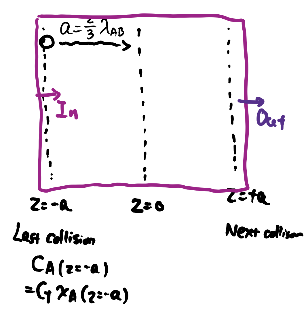
- We also have the average distance \(a\) to one plane from last collision: \[ a = \frac{2}{3}\lambda_{AB} \]
Kinetic theory – mass transfer
When there is only molecular diffusion (no convection), at plane \(z=0\), the flux can be described by:
We can now link \(D_{AB}\) to microscopic properties!
Kinetic theory of diffusivity – conclusion
Results:
\[ D_{AB} = \frac{1}{3} \overline{u} \lambda_{A,B} \]
- \(\overline{u}\): average molecular velocity
- \(\lambda\): mean free path between collisions
Assumptions:
- Rigid sphere type molecules (what are they?)
- No interaction upon collisions
- Collisions are elastic (momentum conserved)
- Good for dilute gases (low \(P\))
- Not accurate otherwise
Molecular diffusivity – Chapman-Enskog theory
We can take real interaction between molecules into the kinetic theory!
\[\begin{align} D_{AB} &= \frac{1.8583\times{}10^{-7} T^{3/2}} {p_T \sigma_{AB}^2 \Omega_{D, AB}} \left(\frac{1}{m_A} + \frac{1}{m_B} \right)^{\frac{1}{2}} \\ &\propto \frac{T^{\frac{3}{2}}}{p_T} \left(\frac{1}{m_A} + \frac{1}{m_B} \right)^{\frac{1}{2}} \end{align}\]- \(m_A\), \(m_B\), molecular weight
- \(\sigma_{AB}\): average collision radius between A and B
- \(\Omega_{D, AB}\): Lennard-Jones collision integral
- \(\Omega_{D, AB}=1\) for elastic collision
- Chapman-Enskog theory accounts for non-elastic collision using \(\Omega_{D, AB}\neq1\)
Chapman-Enskog theory: how to use
\[\begin{align} D_{AB} = \frac{1.8583\times{}10^{-7} T^{3/2}} {p_T \sigma_{AB}^2 \Omega_{D, AB}} \left(\frac{1}{m_A} + \frac{1}{m_B} \right)^{\frac{1}{2}} \end{align}\]The Chapman-Enskog theory formula in Geankoplis book need to use the following units:
- \(T\): absolute temperature in \(\text{K}\)
- \(m_A\), \(m_B\): molecular weight in \(\text{kg} \cdot (\text{kg mol})^{-1}\) or \(\text{g} \cdot (\text{g mol})^{-1}\)
- \(p_T\): absolute pressure in \(\text{atm}\)
- \(\sigma_{AB}\): average collision diameter in Å
- \(\Omega_{D, AB}\): collision integral (dimensionless)
Resulting \(D_{AB}\) is in \(\text{m}^2 \cdot \text{s}^{-1}\)
Chapman-Enskog theory & Lennard-Jones potential
- Parameters \(\sigma_{AB}\) and \(\Omega_{D, AB}\) can be derived using Lennard-Jones (LJ) potential
- LJ potential described the interaction energy \(U_{AB}\) between 2 molecules at distance \(r\) follows:
How to get the parameters from table:
- \(\sigma_{AB} = (\sigma_{A} + \sigma_{B})/2\)
- \(\epsilon_{AB} = \sqrt{\epsilon_A \epsilon_B}\)
- \(\Omega_{D, AB}\): get interpolated table values as function of \(T^*=k_B T / \epsilon_{AB}\)
Note
Check online course materials for the \(\Omega_{D, AB}\) table!
Molecular diffusivity theory – Fuller method
The Chapman Enskog theory can be difficult to use, engineers need some simplied empirical rules.
\[\begin{align} D_{AB} &= \frac{1.0\times{}10^{-7} T^{1.75} }{p_T \left[ (\sum \nu_A)^{1/3} + (\sum \nu_B)^{1/3}\right]^2} \left(\frac{1}{m_A} + \frac{1}{m_B} \right)^{\frac{1}{2}} \\ &\propto \frac{T^{1.75}}{p_T} \end{align}\]- Mainly to overcome the complicated estimation of \(\Sigma_{D, AB}\) in Chapman-Enskog Theory
- \(\sum \nu_i\) sum of structural volume increments
- \(\sum \nu_i\) can be estimated from individual atoms
- Easier to use than the Chapman-Enskog Theory, but less accurate
Fuller method: how to use
\[\begin{align} D_{AB} = \frac{1.0\times{}10^{-7} T^{1.75} }{p_T \left[ (\sum \nu_A)^{1/3} + (\sum \nu_B)^{1/3}\right]^2} \left(\frac{1}{m_A} + \frac{1}{m_B} \right)^{\frac{1}{2}} \end{align}\]The Fuller method formula in Geankoplis book need to use the following units:
- \(T\): absolute temperature in \(\text{K}\)
- \(m_A\), \(m_B\): molecular weight in \(\text{kg} \cdot (\text{kg mol})^{-1}\) or \(\text{g} \cdot (\text{g mol})^{-1}\)
- \(p_T\): absolute pressure in \(\text{atm}\)
- \(\nu_{A}\), \(\nu_{B}\): structural volume increments (dimensionless)
Resulting \(D_{AB}\) is in \(\text{m}^2 \cdot \text{s}^{-1}\)
How to use the Fuller method from a table
We need to determine \(\sum \nu_A\) and \(\sum \nu_B\), Check Table 6.2-2 of Geankoplis 4th ed.
- \(\sum \nu_i\) are dimensionless numbers
- For known gases in the table, use its value in the table
- Air: \(\nu = 20.1\)
- O\(_2\): \(\nu = 16.6\)
- For an unknown gas, use its chemical composition
- For chemical formula \(\text{C}_x \text{H}_y \text{O}_z\), \[ \sum \nu(\text{C}_x \text{H}_y \text{O}_z) = \nu(\text{C}) \cdot x + \nu(\text{H}) \cdot y + \nu(\text{O}) \cdot z \]
Estimating \(D_{AB}\) at different \((T, P)\)
For the same pair of (A, B), both the Chapman-Enskog and Fuller methods have the same form \[ D_{AB} \propto \frac{T^n}{P} \]
This means we can find one existing \(D_{AB}\) value from table and extrapolate: \[ \frac{D_{AB}\vert_1}{D_{AB}\vert_2} = \left(\frac{T_1}{T_2}\right)^{n} \left( \frac{P_2}{P_1} \right) \]
Fuller method is often used in chemical engineering, where \(n=1.75\).
Example 1: Chapman-Enskog theory vs Fuller method
Question: calculate the diffusivity \(D_{AB}\) for methan–ethan system at 313 K and 1 atm.
Chapman-Enskog Theory
- \(m_A=16.04\), \(m_B=30.07\)
- \(\rho_A (Å)=3.822\), \(\rho_B (Å)=4.418\)
- \(\epsilon_A = k_B * (137\ \text{K})\), \(\epsilon_B = k_B * (230\ \text{K})\)
- \(\Omega_{D, AB} = 1.125\) in this case
Fuller Method
- \(m_A=16.04\), \(m_B=30.07\)
- \(\nu(\text{C})=16.5\), \(\nu(\text{H})=1.98\)
The experimental value at this condition is \(D_{AB}=1.84\times 10^{-5}\ \text{m}^2\cdot s^{-1}\). Compare the percent errors in both methods.
Summary
- Diffusivity \(D_{AB}\) value is the key to solve the transport problem in gases
- \(D_{AB}\) can be measured from experiments, but not exhaustively
- Several theories predict the value for \(D_{AB}\) with certain accuracy
- Chapman-Enskog theory and Fuller method both have \(D_{AB}\propto T^n/P\) form
- Fuller method is more often used as it can approximate \(D_{AB}\) solely by taking values from tables