---
title: "CHE 318 Lecture 04"
subtitle: "Molecular Diffusivity: Theories and Measurement"
author: "Dr. Tian Tian"
date: "2026-01-12"
format:
html: {}
revealjs:
output-file: slides.html
pdf:
output-file: L04.pdf
---
::: {.content-visible when-format="html" unless-format="revealjs"}
::: {.callout-note}
- Slides 👉 [Open presentation🗒️](./slides.html)
- PDF version of course note 👉 [Open in pdf](./L04.pdf)
- Handwritten notes 👉 [Open in pdf](./public/L04_annotated.pdf)
:::
:::
::: {.content-visible when-format="revealjs"}
::: {.callout-note}
- **Course Website Updated!**
[https://tiangroup-uofa.github.io/che318-mass-transfer/](https://tiangroup-uofa.github.io/che318-mass-transfer/)
<div style="width: 100%; text-align: center;">
<img
src="https://quickchart.io/qr?text=https://tiangroup-uofa.github.io/che318-mass-transfer/&size=250"
alt="QR Code"
style="width: 150px; height: 150px; display: block; margin: 0 auto;"
/>
</div>
:::
:::
## Recap
- **General solution** for diffusion binary mixture gas systems ($N_B = k N_A$)
- $k = -1$ reduces to EMCD solution
- Total flux $N_A$ is EMCD flux times a coefficient
```{=tex}
\begin{align}
N_A = \frac{ c_T D_{AB}}{(z_2 - z_1)}
\left(\frac{N_A}{N_A + N_B}\right)
\ln\!\left[\dfrac{
\frac{N_A}{N_A + N_B} - x_{A2}}
{\frac{N_A}{N_A + N_B} - x_{A1}}
\right]
\end{align}
```
- Brief discussion about diffusivity measurement: two-bulb setup
## Demonstration of general solution
```{=html}
<iframe width="100%" height="800"
src="../../scripts/L03_xa_profile.html" title="Webpage example"></iframe>
```
## Interaction time!
[participation link](https://app.wooclap.com/318L04?from=instruction-slide)
*Results and comments to be published after the class*
::: {.content-visible when-format="revealjs"}
---
## Convection-driven flux change
{#fig-na-comp width="100%"}
:::
::: {.content-visible when-format="html" unless-format="revealjs"}
---
## Detailed explanation for convection-driven flux change
::: {.callout-note}
Advanced topic, not shown in presentation
:::
The ratio between total flux in general solution $N_A(\text{gen})$ and $N_A(\text{EMCD})$ can be written as:
```{=tex}
\begin{align}
\frac{N_A(\text{gen})}{N_A(\text{EMCD})}
&= \frac{s \ln\! \left[
\frac{s - x_{A2}}{s - x_{A1}}
\right]}{x_{A1} - x_{A2}} \\
&= \frac{s \ln\! \left[
\frac{s - x_{A2}}{s - x_{A1}}
\right]}{(s - x_{A2}) - (s - x_{A1})} \\
&= \frac{s}{\text{LM}(s-x_A)}
\end{align}
```
where $\text{LM}(u)$ is the log-mean function (similar treatment in [Lecture 2](../L02)), and $s = N_A / (N_A + N_B)$.
There are several limiting cases. Let's assume $x_{A1} > x_{A2}$ for simplicity, and there is a real solution to the $N_A(\text{gen})$
1. $s > x_{A1}$:
$s - x_{A1}$ and $s - x_{A2}$ must be both positive to ensure a
solution. Therefore $\text{LM}(s-x_A) < s$. We know that
$N_A(\text{gen})>N_A(\text{EMCD})$.
- Example: diffusion through stagnant B ($s = 1$)
In this case $\text{LM}(s-x_A) = \text{LM}(x_B)$, we can conclude that the diffusion through stagnant B case **always enhances** total flux compared with EMCD.
A signature of such transport is the $x_A(z)$ profile is **concave**, as shown in @fig-na-comp (a).
2. $s < 0$:
$s - x_{A2}$ and $s - x_{A1}$ are be both negative. Therefore $|\text{LM}(s-x_A)| > s$. We know that
$N_A(\text{gen})<N_A(\text{EMCD})$, but $N_A$ is still positive.
- Example: counter $N_B$ flux ($N_B/N_A < -1$)
The opposite direction of $N_B$ **attenuates** the molar flux of A. A signature of such transport is the $x_A(z)$ profile is **convex**, as shown in @fig-na-comp (b).
3. $0 < s < x_2$:
$s - x_{A2}$ and $s - x_{A1}$ are be both negative. Since $s >0$, we actually can have $N_A < 0$!
Such situation may be counter-intuitive but the solution is physically valid, as the only solution to satisfy such criteria is $N_B < 0$ and $N_A < 0$ at the same time.
As we cannot directly compare $s$ and $\text{LM}(s-x_A)$ in this case, $|N_A(\text{gen})|$ can be either smaller or larger than $N_A(\text{EMCD})$, as shown in @fig-na-comp (c) and (d).
4. $x_2 < s < x_1$:
The expression inside the logarithm is negative and we do not have a real solution to the general equation for $N_A$.
{#fig-na-comp width="100%"}
:::
---
## Learning outcomes {.center}
After this lecture, you will be able to:
- **Recall** major theories used to estimate molecular diffusivity.
- **Describe** how the diffusivity $D_{AB}$ changes with temperature and pressure.
- **Apply** tabulated reference data to estimate diffusivity values.
- **Formulate** governing equations for common diffusivity-measurement scenarios.
---
## Let's look at the general mass transfer equation (again)
$$
N_A = \frac{D_{AB} c_T}{(z_2 - z_1)}
s
\ln\!\left[\dfrac{
s - \frac{c_{A2}}{c_T}}
{s - \frac{c_{A1}}{c_T}}
\right]
\quad
s = \frac{N_A}{N_A + N_B}
$$
What values do we know from the system setup?
- Geometry: $z_1$, $z_2$, $c_{A1}$, $c_{A2}$, $c_T$
- Chemical reaction stoichiometry: $k$
What else value(s) do we need to solve $N_A$?
- $D_{AB}$: generally $D_{AB}(z) = \text{Const}$
- But $D_{AB}=f(T, P, \cdots)$
---
## Motivation to have theory about diffusivity {.center}
- Solving the general solution for gas mass transfer requires parameter $D_{AB}$ (and $D_{BA}$)!
- Measuring every $D_{AB}$ pair for gases is tedious
- $D_{AB}$ is dependent on conditions $T, P$
- We need to have theories that can **predict** diffusivity $D_{AB}$ **without** doing all pair experiments and all $(T, P)$ conditions!
- In the lease case, the theory should allow extrapolating a measured $D_{AB}(T_1, P_1)$ to $D_{AB}(T_2, P_2)$
---
## Molecular diffusivity theory -- kinetic theory
In dilute gas regime ($p_T \approx \text{atm}$), the kinetic behaviour
of gas molecules can be described using kinetic theory. A few
assumptions are made:
1. Interdiffusion between A and B are dominated by **collision** between molecules (low $p_T$ 👉 **only 2** molecules can collide at the same time)
2. The molecules are rigid spheres having particle masses $m_A$, $m_B$ and diameters $d_A$ and $d_B$
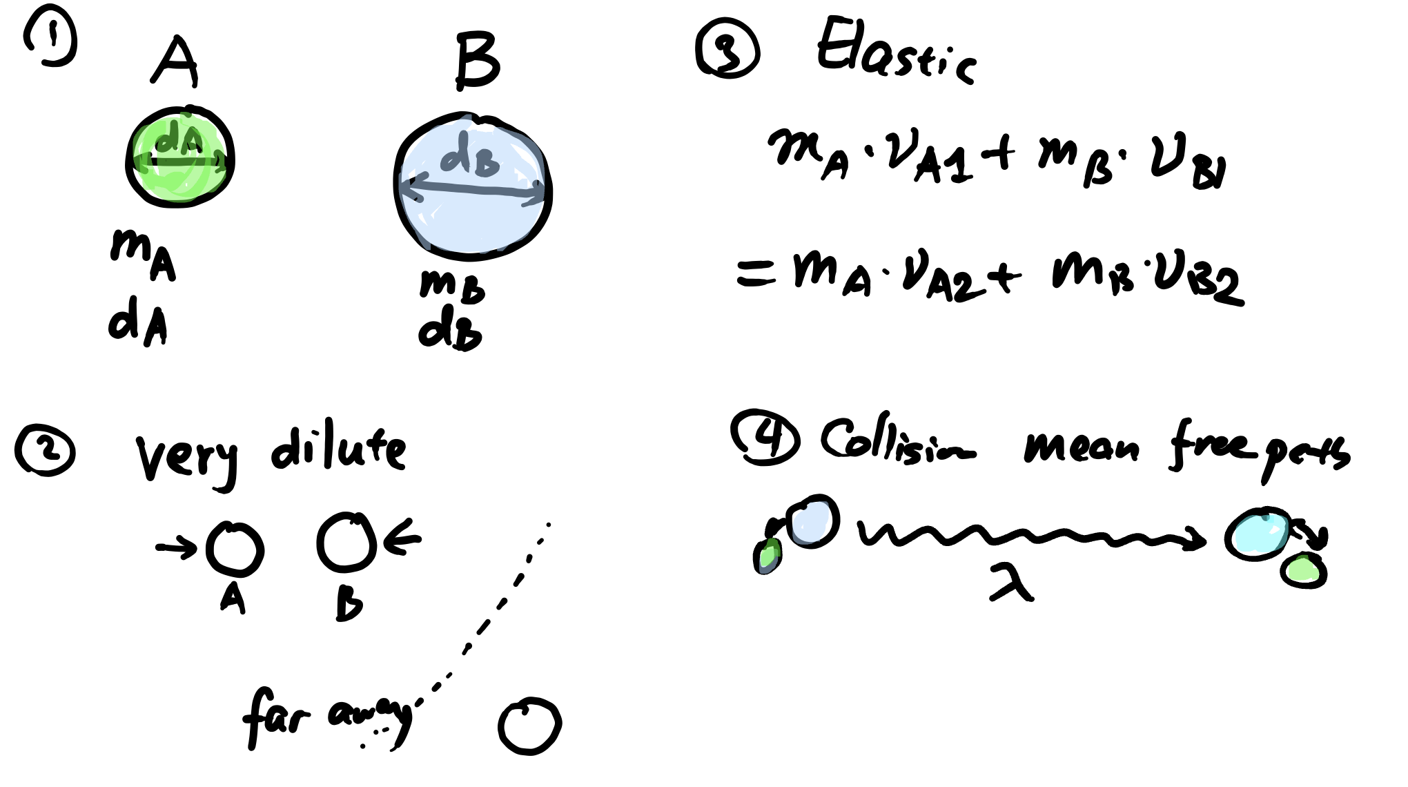{width="80%"}
## Kinetic theory -- key results
There are some results from the kinetic theory:
^[adapted from *BSL Transport Phenomena ch 17.3*]
::: {.columns}
::: {.column width="50%"}
1. Mean molecular speed $\overline{u}$
$$
\overline{u} = \sqrt{\frac{8 k_B T}{\pi \overline{m_{AB}}}}
$$
2. Mean free path (between collisions): $\lambda_{A,B}$
$$
\lambda_{AB}=\frac{1}{\sqrt{2} \pi d_{AB}^2 c_T}
$$
:::
::: {.column width="50%"}
3. Frequency of molecule A colliding with wall ($Z$, unit $\text{m}^{-2}\cdot \text{s}^{-1}$):
$$
Z_A = \frac{1}{4} c_A \overline{u}
$$
where $d_{AB} = \frac{d_A + d_B}{2}$, $m_{AB}^{-1} = m_{A}^{-1} + m_B^{-1}$, $k_B$ is the Boltzmann constant
4. We also have the average distance $a$ to one plane from last collision:
$$
a = \frac{2}{3}\lambda_{AB}
$$
:::
:::
---
## Kinetic theory -- mass transfer
When there is only molecular diffusion (no convection), at plane $z=0$, the flux can be described by:
::: {.columns}
::: {.column width="60&"}
```{=tex}
\begin{align}
J_{Az}^*\vert_{z=0} &= \text{[In]}\vert_{z=-a} - \text{[Out]}\vert_{z=+a} \\
&= \frac{1}{4} c_T [x_A \overline{u}]\vert_{z=-a} \\
&- \frac{1}{4} [c_T x_A \overline{u}]\vert_{z=+a}\\
&= -\frac{1}{4} c_T \cdot 2a \cdot \overline{u} \frac{d x_A}{dz} \\
&= -D_{AB} c_T \frac{dx_A}{dz}
\end{align}
```
We can now link $D_{AB}$ to microscopic properties!
:::
::: {.column width="40%"}
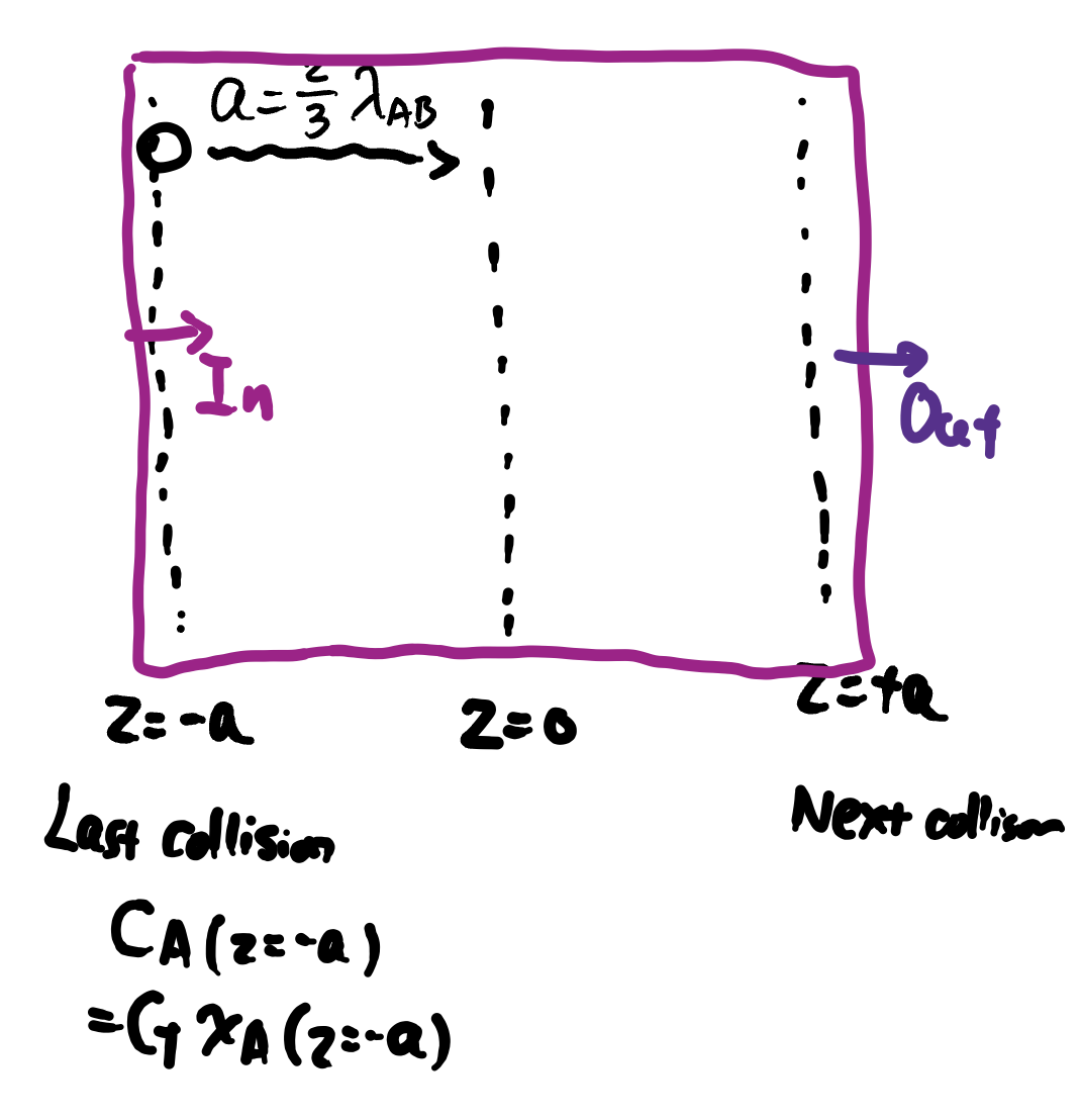{width="80%"}
:::
:::
---
## Kinetic theory of diffusivity -- conclusion
::: {.columns}
::: {.column width="50%"}
Results:
$$
D_{AB} = \frac{1}{3} \overline{u} \lambda_{A,B}
$$
- $\overline{u}$: average molecular velocity
- $\lambda$: mean free path between collisions
:::
:::{.column width="50%"}
Assumptions:
- Rigid sphere type molecules (what are they?)
- No interaction upon collisions
- Collisions are elastic (momentum conserved)
- Good for dilute gases (low $P$)
- Not accurate otherwise
:::
:::
---
## Molecular diffusivity -- Chapman-Enskog theory
We can take real interaction between molecules into the kinetic theory!
```{=tex}
\begin{align}
D_{AB} &= \frac{1.8583\times{}10^{-7} T^{3/2}}
{p_T \sigma_{AB}^2 \Omega_{D, AB}} \left(\frac{1}{m_A} + \frac{1}{m_B} \right)^{\frac{1}{2}} \\
&\propto \frac{T^{\frac{3}{2}}}{p_T} \left(\frac{1}{m_A} + \frac{1}{m_B} \right)^{\frac{1}{2}}
\end{align}
```
- $m_A$, $m_B$, molecular weight
- $\sigma_{AB}$: average collision radius between A and B
- $\Omega_{D, AB}$: Lennard-Jones collision integral
- $\Omega_{D, AB}=1$ for elastic collision
- Chapman-Enskog theory accounts for non-elastic collision using $\Omega_{D, AB}\neq1$
---
## Chapman-Enskog theory: how to use
```{=tex}
\begin{align}
D_{AB} = \frac{1.8583\times{}10^{-7} T^{3/2}}
{p_T \sigma_{AB}^2 \Omega_{D, AB}} \left(\frac{1}{m_A} + \frac{1}{m_B} \right)^{\frac{1}{2}}
\end{align}
```
The Chapman-Enskog theory formula in *Geankoplis book* need to use the following units:
- $T$: absolute temperature in $\text{K}$
- $m_A$, $m_B$: molecular weight in $\text{kg} \cdot (\text{kg mol})^{-1}$ or $\text{g} \cdot (\text{g mol})^{-1}$
- $p_T$: absolute pressure in $\text{atm}$
- $\sigma_{AB}$: average collision diameter in Å
- $\Omega_{D, AB}$: collision integral (dimensionless)
Resulting $D_{AB}$ is in $\text{m}^2 \cdot \text{s}^{-1}$
---
## Chapman-Enskog theory & Lennard-Jones potential
- Parameters $\sigma_{AB}$ and $\Omega_{D, AB}$ can be derived using Lennard-Jones (LJ) potential
- LJ potential described the interaction energy $U_{AB}$ between 2 molecules at distance $r$ follows:
```{=tex}
\begin{align}
U_{AB}(r) = 4\epsilon_{AB}\left[
(\frac{\sigma_{AB}}{r})^{12} - (\frac{\sigma_{AB}}{r})^{6}
\right]
\end{align}
```
How to get the parameters from table:
- $\sigma_{AB} = (\sigma_{A} + \sigma_{B})/2$
- $\epsilon_{AB} = \sqrt{\epsilon_A \epsilon_B}$
- $\Omega_{D, AB}$: get interpolated table values as function of $T^*=k_B T / \epsilon_{AB}$
::: {.callout-note}
Check online [course materials]() for the $\Omega_{D, AB}$ table!
:::
---
## Molecular diffusivity theory -- Fuller method
The Chapman Enskog theory can be difficult to use, engineers need some simplied empirical rules.
```{=tex}
\begin{align}
D_{AB} &= \frac{1.0\times{}10^{-7} T^{1.75} }{p_T \left[ (\sum \nu_A)^{1/3} + (\sum \nu_B)^{1/3}\right]^2}
\left(\frac{1}{m_A} + \frac{1}{m_B} \right)^{\frac{1}{2}} \\
&\propto \frac{T^{1.75}}{p_T}
\end{align}
```
- Mainly to overcome the complicated estimation of $\Sigma_{D, AB}$ in Chapman-Enskog Theory
- $\sum \nu_i$ sum of structural volume increments
- $\sum \nu_i$ can be estimated from individual atoms
- Easier to use than the Chapman-Enskog Theory, but less accurate
---
## Fuller method: how to use
```{=tex}
\begin{align}
D_{AB} = \frac{1.0\times{}10^{-7} T^{1.75} }{p_T \left[ (\sum \nu_A)^{1/3} + (\sum \nu_B)^{1/3}\right]^2}
\left(\frac{1}{m_A} + \frac{1}{m_B} \right)^{\frac{1}{2}}
\end{align}
```
The Fuller method formula in *Geankoplis book* need to use the following units:
- $T$: absolute temperature in $\text{K}$
- $m_A$, $m_B$: molecular weight in $\text{kg} \cdot (\text{kg mol})^{-1}$ or $\text{g} \cdot (\text{g mol})^{-1}$
- $p_T$: absolute pressure in $\text{atm}$
- $\nu_{A}$, $\nu_{B}$: structural volume increments (dimensionless)
Resulting $D_{AB}$ is in $\text{m}^2 \cdot \text{s}^{-1}$
## How to use the Fuller method from a table
We need to determine $\sum \nu_A$ and $\sum \nu_B$,
*Check Table 6.2-2 of Geankoplis 4th ed*.
- $\sum \nu_i$ are **dimensionless** numbers
- For known gases in the table, use its value in the table
- Air: $\nu = 20.1$
- O$_2$: $\nu = 16.6$
- For an unknown gas, use its chemical composition
- For chemical formula $\text{C}_x \text{H}_y \text{O}_z$,
$$
\sum \nu(\text{C}_x \text{H}_y \text{O}_z)
= \nu(\text{C}) \cdot x + \nu(\text{H}) \cdot y + \nu(\text{O}) \cdot z
$$
## Estimating $D_{AB}$ at different $(T, P)$
For the same pair of (A, B), both the Chapman-Enskog and Fuller methods have the same form
$$
D_{AB} \propto \frac{T^n}{P}
$$
This means we can find one existing $D_{AB}$ value from table and extrapolate:
$$
\frac{D_{AB}\vert_1}{D_{AB}\vert_2}
= \left(\frac{T_1}{T_2}\right)^{n}
\left(
\frac{P_2}{P_1}
\right)
$$
Fuller method is often used in chemical engineering, where $n=1.75$.
---
## Example 1: Chapman-Enskog theory vs Fuller method
Question: calculate the diffusivity $D_{AB}$ for methan--ethan system at 313 K and 1 atm.
::: {.columns}
::: {.column width="50%"}
#### Chapman-Enskog Theory
- $m_A=16.04$, $m_B=30.07$
- $\rho_A (Å)=3.822$, $\rho_B (Å)=4.418$
- $\epsilon_A = k_B * (137\ \text{K})$, $\epsilon_B = k_B * (230\ \text{K})$
- $\Omega_{D, AB} = 1.125$ in this case
:::
::: {.column width="50%"}
#### Fuller Method
- $m_A=16.04$, $m_B=30.07$
- $\nu(\text{C})=16.5$, $\nu(\text{H})=1.98$
:::
:::
The experimental value at this condition is $D_{AB}=1.84\times 10^{-5}\ \text{m}^2\cdot s^{-1}$. Compare the percent errors in both methods.
::: {.content-visible when-format="html" unless-format="revealjs"}
---
## Solution to example 1:
```{python}
#| echo: false
import marimo as mo
def chapman(ma, mb, T, p, sig_a, sig_b, Omega):
coeff = 1.8583e-7
numerator = coeff * T ** 1.5
denominator = p * ((sig_a + sig_b) / 2) ** 2 * Omega
mass_inv = (1/ma + 1/mb) ** 0.5
return numerator / denominator * mass_inv
def fuller(ma, mb, T, p, nu_a, nu_b):
coeff = 1.0e-7
numerator = coeff * T ** 1.75
denominator = p * (nu_a ** (1/3) + nu_b ** (1/3)) ** 2
mass_inv = (1/ma + 1/mb) ** 0.5
return numerator / denominator * mass_inv
def nu_ch(x_c, x_h):
nu_c = 16.5
nu_h = 1.98
return nu_c * x_c + nu_h * x_h
def calculate():
ma = 16.04
mb = 30.07
symb_a = (1, 4)
symb_b = (2, 6)
_T = 313
_p = 1.0
sig_a = 3.822
sig_b = 4.418
Omega = 1.125
v_chap = chapman(ma, mb, _T, _p, sig_a, sig_b, Omega)
v_fuller = fuller(ma, mb, _T, _p, nu_ch(*symb_a), nu_ch(*symb_b))
v_real = 1.84e-5
output = mo.vstack([
mo.md(f"""**Chapman-Enskog Theory**:
- Diffusivity (m^2/s) = {v_chap:.3e}
- Percentage error: {abs((v_chap - v_real) / v_real) * 100:.2f}%
"""),
mo.md(f"""
**Fuller Method**:
- Diffusivity (m^2/s) = {v_fuller:.3e}
- Percentage error: {abs((v_fuller - v_real) / v_real) * 100:.2f}%
"""
)])
return output
calculate()
```
:::
---
## Summary
- Diffusivity $D_{AB}$ value is the key to solve the transport problem in gases
- $D_{AB}$ can be measured from experiments, but not exhaustively
- Several theories predict the value for $D_{AB}$ with certain accuracy
- Chapman-Enskog theory and Fuller method both have $D_{AB}\propto T^n/P$ form
- Fuller method is more often used as it can approximate $D_{AB}$ solely by taking values from tables


