MATE 664 Lecture 08

Numerical Solution To Diffusion Problems & Atomic Models for Diffusion

Dr. Tian Tian

2026-01-28

Recap of Lecture 07

Key ideas from last lecture:

  • Analytical solution to diffusion problems (infinite domain)
    • Semi-infinite (half-half) solution
    • Line / point source solution
    • Superimposition method
  • Separation of variables method (finite / bounded domain)
  • Laplace transform (will not be covered in exam)

Learning Outcomes

After today’s lecture, you will be able to:

  • Describe detail ideas behind the numerical / finite-difference solution to diffusion problems
  • Recall basic formalism of discrete differential equation
  • Apply numerical methods for diffusion problems and diffusivity extraction
  • Analyze atomic origin of diffusion

Numerical Method For Diffusion Equation

In many cases the analytical solutions to a diffusion equation is hard / impossible to obtain, due to:

  • complicated B.C. I.C.s
  • non-uniform or anisotropic diffusivities
  • existing of multiple phases during diffusion
  • inhomogeneous temperature distribution
  • … other experimental conditions you can think of

We need numerical methods for these situations!

Finite Difference Method

For 1D problem 👉 use the finite difference (FD) method first proposed by Euler.

FD In A Nutshell

To solve the diffusion equation, we need to discretize spatial and temporal domains into “grids”.

Derivatives By Finite Difference

In Fick’s second law, the required derivatives and their finite-difference approximations are summarized below. The concentration on grid is \(c(i,j)\), where \(i\) indexes space and \(j\) indexes time.

derivative finite-difference approximation scheme
\(\displaystyle \frac{\partial c}{\partial t}\) \(\displaystyle \frac{c(i,\,j+1) - c(i,\,j)}{\Delta t}\) forward (time)
\(\displaystyle \frac{\partial c}{\partial x}\) \(\displaystyle \frac{c(i+1,\,j) - c(i-1,\,j)}{2\Delta x}\) central (space)
\(\displaystyle \frac{\partial^2 c}{\partial x^2}\) \(\displaystyle \frac{c(i+1,\,j) - 2c(i,\,j) + c(i-1,\,j)}{(\Delta x)^2}\) central (space)

Solving Diffusion Equation: Method of Lines (MOL)

Fick’s second law is PDE which is hard to integrate directly. Method of lines use the following strategies:

  • Discretize space only
  • Keep time continuous
  • Convert PDE into a system of ODEs in time

After spatial discretization 👉 ODE in temporal domain

\[\begin{align} \frac{d c(i,t)}{d t} = D \frac{c(i+1,t) - 2c(i,t) + c(i-1,t)}{(\Delta x)^2} \end{align}\]

Each spatial node \(i\) (line) corresponds to one ODE, hence the name.

MOL Algorithm (Explicit Time Marching)

  1. Define spatial grid with \(x_i\) (\(N\) points), choose \(\Delta x\)
  2. Apply boundary conditions at \(i=0\) and \(i=N\)
  3. Discretize spatial derivatives using central difference
  4. Obtain ODE system for \(c(i,t)\)
  5. Choose time step \(\Delta t\)
  6. Advance solution in time using forward Euler:
\[\begin{align} c(i,j+1) &= c(i,j) + \Delta t \, \frac{d c(i,t)}{d t} \\ &= c(i,j) + \Delta t \cdot D \frac{c(i+1,t) - 2c(i,t) + c(i-1,t)}{(\Delta x)^2} \end{align}\]

Things To Check In FD Scheme

  • Grid stability condition

    \[\Delta t \le \frac{(\Delta x)^2}{2D}\]

  • Convergence: are \(\Delta t\) and \(\Delta x\) small enough?

  • Numerical precision: stiff diffusion problems (e.g. Nernst-Planck) may require higher numerical precision

  • Boundary condition implementation

  • Conservation

  • Solving steady state problem (Laplace problem) can be non-trivial

Implementation and Multi-Dimensional Extensions

  • Open-source implementation (FD + MOL)
    • Python + NumPy for spatial discretization
    • scipy.integrate.solve_ivp for time integration
  • Open-source PDE solvers
    • Finite volume method (FVM): OpenFOAM (C++), FiPy (Python)
    • Finite element method (FEM) FEniCS (Python)
  • Commercial multiphysics solvers
    • FEM: COMSOL Multiphysics
    • FVM: ANSYS
  • Development of solvers is a hot field for engineering!

Some Skeleton Code in Python

MOL can usually be implemented using pure Python in less than 20 lines (really not that difficult!)

FD Numerical Method Demo

How do FD compare with analytical solution?

Estimating Diffusivity: Example 1

The first diffusivity in metal was presented in 1894 by Roberts-Austen using diffusion of Au in liquid Pb. (See review by Mehrer and Stolwijk, Diffusion Fundamentals, 2008, 1, 1-32).

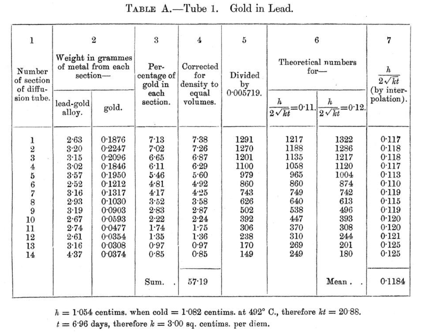
The experiment is basically a solid Au-Pd alloy cylinder diffusing into semi-infinite molten Pd at \(T\)=492 ℃, as the geometry below. Experiment weight fraction of Au was determined by precision scales on sections of cylinder after \(t=6.96\) days. Can we verify his results of diffusivity (\(\tilde{D}=3.00\) cm\(^2\)d\(^{-1}\))?

Roberts-Austen Experiment: Original Data & Setup

See Bakerian Lecture: On the Diffusion of Metals. Roberts-Austen

Roberts-Austen’s original experimental data

Setup scheme

Roberts-Austen Experiment: Fitting

More Complex Situation: Multiphase Interdiffusion

  • Diffusion couple experiments often cross phase boundaries
    • single-phase → two-phase → single-phase regions
    • composition is no longer a single-valued function of chemical potential

Example 1: Ir–Re diffusion couple annealed at 2400°C (adapted from MIT KOM course)

  • How many discontinuities?

More Complex Situation: Multiphase Interdiffusion

Example 2: Os-W diffusion couple annealed at 2200°C (adapted from MIT KOM course)

  • How many discontinuities?
  • How do we model these problems?
  • See packages like pyDiffusion

Introduction to Atomic Models of Diffusion

Motivation: Predicting \(D\) From Atomistic Simulations

  • We know from experiments how to extract the \(D\) (or \(\tilde{D}\)) very well
  • But how are the diffusivities coming from atomic models?
  • Can we predict \(D\) from some calculations?

Diffusion: Bridging Atomic and Macroscopic Pictures

Two major achievements in 20th century

  • Explanation of Brownian motion (Einstein)
    • macroscopic diffusion emerges from random atomic motion
    • link between mean-square displacement and diffusivity
  • Atomic interpretation of Fick’s laws
    • diffusion coefficient related to jump frequency and jump distance
    • connects lattice-scale mechanisms to continuum transport equations

Mean Squared Displacement (Brownian Motion Picture)

A particle undergoes a sequence of thermally activated jumps

  • jump displacement for \(k\)-th step: \(\vec{r}_k\)
  • after \(N_s\) jumps, total displacement:

\[ \vec{R}(N_s) = \sum_{k=1}^{N_s} \vec{r}_k \]

  • What is the mean displacement \(\langle R \rangle\)? (it’s zero!)

Mean squared displacement (MSD):

\[ \langle R^2(N_s) \rangle = \left\langle \vec{R}(N_s)\cdot \vec{R}(N_s) \right\rangle \]

MSD: Expansion and Randomness Assumption

Expand the dot product:

\[ R^2(N_s) = \sum_{k=1}^{N_s} |\vec{r}_k|^2 + 2\sum_{k=1}^{N_s-1}\sum_{m=k+1}^{N_s} \vec{r}_k \cdot \vec{r}_m \]

If successive jumps are uncorrelated (random directions):

\[ \langle \vec{r}_k \cdot \vec{r}_m \rangle = 0 \quad (k\neq m) \]

Then

\[ \langle R^2(N_s) \rangle = N_s \langle r^2 \rangle \]

where \(\langle r^2 \rangle\) is the mean squared jump distance.

Random Jump MSD from Continuum Diffusion

Consider diffusion from a point source in 3D into infinite space. The concentration at each \(r\) at any time \(t\) is \(c(r, t)\)

Define MSD as the normalized second moment of \(c(r, t)\)

\[ \langle R^2(t)\rangle = \frac{\int_0^\infty r^2\,c(r,t)\,4\pi r^2\,dr}{\int_0^\infty c(r,t)\,4\pi r^2\,dr} \]

Luckily, the solution to \(c(r, t)\) was already known in 1905 as Gaussian (also from last lecture):

\[ c(r, t) = \frac{N}{{\sqrt{4 \pi Dt}}^3} \exp\!(-\frac{r^2}{4Dt}),\qquad r^2 = x^2 + y^2 + z^2 \]

Einstein Diffusion Equation From Continuum Diffusio

Use the Gaussian form, Einstein showed for 3D random jump, we have

\[ \langle R^2(t)\rangle = 6Dt \]

More generally in \(d\) dimensions:

\[ \langle R^2(t)\rangle = 2d\,Dt \]

  • This is known as Einstein diffusion equation
  • Links atomic motion (Brownian motion, \(<R^2>\)) to continuum diffusion (\(D\))

Diffusion From Random Walk Model

1D random walk with step \(\pm 1\) (site index \(n\))

Constraints after \(N_\tau\) steps:

\[ N_R - N_L = n,\quad N_R + N_L = N_\tau \]

Number of ways (binomial):

\[ U(n,N_\tau)=\frac{N_\tau!}{N_R!N_L!} \]

For an unbiased walk \(p_L=p_R=1/2\):

\[ p(n,N_\tau) = \frac{N_\tau!}{N_R!N_L!}\left(\frac12\right)^{N_\tau} \]

Large-step limit gives Gaussian form:

\[ p(n,N_\tau)\propto \exp\!\left(-\frac{n^2}{2N_\tau}\right) \]

Linking Random Walk to Macroscopic \(D\)

Identify:

  • diffusion distance: \(x \sim n\,\Delta x\)
  • number of steps: \(N_\tau \sim \Gamma t\) (jump frequency \(\Gamma\))

From MSD (1D):

\[ \langle x^2(t)\rangle = \langle n^2\rangle (\Delta x)^2 \sim N_\tau (\Delta x)^2 \sim \Gamma t (\Delta x)^2 \]

Compare with Einstein (1D): \(\langle x^2(t)\rangle = 2Dt\)

\[ D = \frac{\Gamma (\Delta x)^2}{2} \qquad \text{(in 1D)} \]

General \(d\)-D form:

\[ D = \frac{\Gamma \langle r^2\rangle}{2d} \]

Summary

  • Numerical solutions to diffusion equations
  • Applying numerical fitting for \(D\)
  • Introducing to atomic picture of diffusivity

Next Steps

  • Understanding the atomic model in liquid and lattices
  • Complex mechanism of lattice diffusion
  • Estimating \(D\) from thermodynamic data