---
title: "MATE 664 Lecture 08"
subtitle: "Numerical Solution To Diffusion Problems & Atomic Models for Diffusion"
author: "Dr. Tian Tian"
date: "2026-01-28"
format:
html: {}
revealjs:
output-file: slides.html
pdf:
output-file: L08.pdf
---
::: {.content-visible when-format="html" unless-format="revealjs"}
::: {.callout-note}
- Slides 👉 [Open presentation🗒️](./slides.html)
- PDF version of course note 👉 [Open in pdf](./L08.pdf)
- Handwritten notes 👉 [Open in pdf](./public/L08_annotated.pdf)
:::
:::
## Recap of Lecture 07 {.center}
Key ideas from last lecture:
- Analytical solution to diffusion problems (infinite domain)
- Semi-infinite (half-half) solution
- Line / point source solution
- Superimposition method
- Separation of variables method (finite / bounded domain)
- Laplace transform (will not be covered in exam)
## Learning outcomes {.center}
After this lecture, you will be able to:
- **Describe** the basic ideas behind finite-difference solutions to diffusion problems
- **Recall** the basic form of discrete differential equations
- **Apply** numerical methods to diffusion problems and diffusivity extraction
- **Analyze** the atomic origin of diffusion
## Numerical method for diffusion equation
In many cases the analytical solutions to a diffusion equation is hard / impossible to obtain, due to:
- complicated B.C. I.C.s
- non-uniform or anisotropic diffusivities
- existing of multiple phases during diffusion
- inhomogeneous temperature distribution
- ... other experimental conditions you can think of
We need numerical methods for these situations!
## Finite difference method
For 1D problem 👉 use the **finite difference** (FD) method first proposed by Euler.
{width="80%"}
## FD in a nutshell
To solve the diffusion equation, we need to **discretize** spatial and
temporal domains into "grids".
{width="80%"}
## Derivatives by finite difference
In Fick's second law, the required derivatives and their finite-difference
approximations are summarized below.
The concentration on grid is $c(i,j)$, where
$i$ indexes space and $j$ indexes time.
| derivative | finite-difference approximation | scheme |
|-----------|----------------------------------|--------|
| $\displaystyle \frac{\partial c}{\partial t}$ | $\displaystyle \frac{c(i,\,j+1) - c(i,\,j)}{\Delta t}$ | forward (time) |
| $\displaystyle \frac{\partial c}{\partial x}$ | $\displaystyle \frac{c(i+1,\,j) - c(i-1,\,j)}{2\Delta x}$ | central (space) |
| $\displaystyle \frac{\partial^2 c}{\partial x^2}$ | $\displaystyle \frac{c(i+1,\,j) - 2c(i,\,j) + c(i-1,\,j)}{(\Delta x)^2}$ | central (space) |
## Solving diffusion equation: method of lines (MOL)
Fick's second law is PDE which is hard to integrate directly. Method of lines use the following strategies:
- Discretize space only
- Keep time continuous
- Convert PDE into a system of ODEs in time
After spatial discretization 👉 ODE in temporal domain
```{=tex}
\begin{align}
\frac{d c(i,t)}{d t}
=
D \frac{c(i+1,t) - 2c(i,t) + c(i-1,t)}{(\Delta x)^2}
\end{align}
```
Each spatial node $i$ (line) corresponds to one ODE, hence the name.
## MOL algorithm (explicit time marching)
1. Define spatial grid with $x_i$ ($N$ points), choose $\Delta x$
2. Apply boundary conditions at $i=0$ and $i=N$
3. Discretize spatial derivatives using central difference
4. Obtain ODE system for $c(i,t)$
5. Choose time step $\Delta t$
6. Advance solution in time using forward Euler:
```{=tex}
\begin{align}
c(i,j+1)
&=
c(i,j)
+
\Delta t \,
\frac{d c(i,t)}{d t} \\
&= c(i,j) + \Delta t \cdot D \frac{c(i+1,t) - 2c(i,t) + c(i-1,t)}{(\Delta x)^2}
\end{align}
```
## Things to check in FD scheme
- Grid stability condition
$$\Delta t \le \frac{(\Delta x)^2}{2D}$$
- Convergence: are $\Delta t$ and $\Delta x$ small enough?
- Numerical precision: stiff diffusion problems (e.g. Nernst-Planck) may require higher numerical precision
- Boundary condition implementation
- Conservation
- Solving steady state problem (Laplace problem) can be non-trivial
## Implementation and multi-dimensional extensions
- Open-source implementation (FD + MOL)
- Python + NumPy for spatial discretization
- `scipy.integrate.solve_ivp` for time integration
- Open-source PDE solvers
- Finite volume method (FVM): OpenFOAM (C++), FiPy (Python)
- Finite element method (FEM) FEniCS (Python)
- Commercial multiphysics solvers
- FEM: COMSOL Multiphysics
- FVM: ANSYS
- Development of solvers is a hot field for engineering!
## Some skeleton code in Python
MOL can usually be implemented using pure Python in less than 20 lines
(really not that difficult!)
```{python}
#| eval: false
from scipy.integrate import solve_ivp

def rhs(t, c, D, dx):
    """ Function to implement right-hand-side FD """
    return delta_c_array

def apply_bc(c):
   """ Function to enforce boundary conditions """
   return modified_c_array

def solve_diffusion(c0, t_span, D, dx):
    """
    high-level diffusion solver
    """
    def rhs_bc(t, c):
        c = apply_bc(c)
        return rhs(t, c, D, dx)

    sol = solve_ivp(
        rhs_bc,
        t_span,
        c0,
        method="RK45"
    )
    return sol
```
## FD numerical method demo
How do FD compare with analytical solution?
```{=html}
<iframe width="100%" height="900"
src="../../scripts/L08_fd_comparison.html" title="Webpage example"></iframe>
```
## Estimating diffusivity: example 1
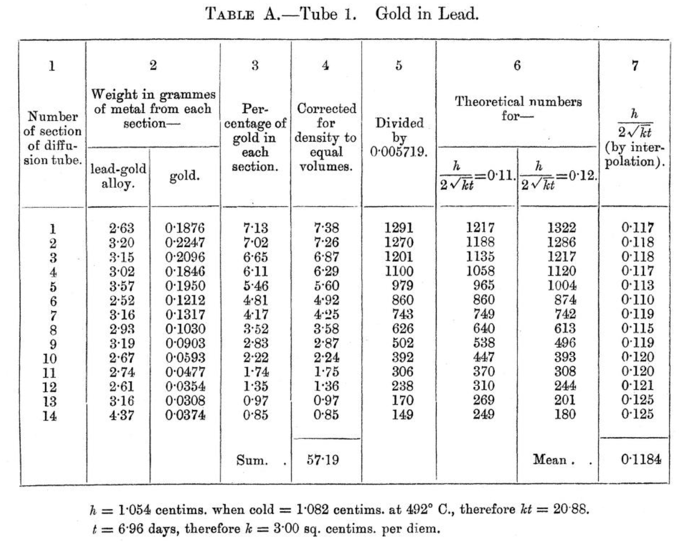
The first diffusivity in metal was presented in 1894 by Roberts-Austen using diffusion of Au in liquid Pb. (See review by _Mehrer and Stolwijk, Diffusion Fundamentals, 2008, 1, 1-32_).
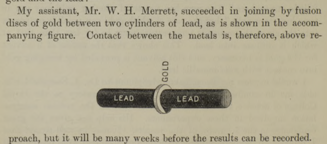
The experiment is basically a solid Au-Pd alloy cylinder diffusing
into semi-infinite molten Pd at $T$=492 ℃, as the geometry
below. Experiment weight fraction of Au was determined by precision scales on sections of cylinder after $t=6.96$ days. Can we verify his results of diffusivity ($\tilde{D}=3.00$ cm$^2$d$^{-1}$)?
{width="50%"}
## Roberts-Austen experiment: original data & setup
See [Bakerian Lecture: On the Diffusion of Metals. Roberts-Austen](https://archive.org/details/philtrans09730582/page/n9/mode/2up)
:::{.columns}
:::{.column}
{width="100%"}
:::
:::{.column}
{width="100%"}
:::
:::
## Roberts-Austen experiment: fitting
```{=html}
<iframe width="100%" height="900"
src="../../scripts/L08_pb_au_diff_fit.html" title="Webpage example"></iframe>
```
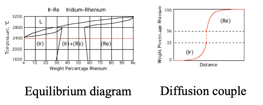
## More complex situation: multiphase interdiffusion
- Diffusion couple experiments often cross phase boundaries
- single-phase → two-phase → single-phase regions
- composition is no longer a single-valued function of chemical potential
Example 1: Ir–Re diffusion couple
annealed at 2400°C (_adapted from MIT KOM course_)
- How many discontinuities?
{width="100%"}
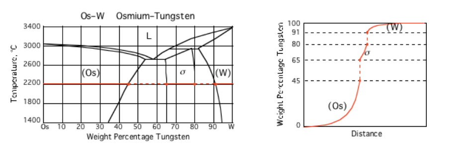
## More complex situation: multiphase interdiffusion
Example 2: Os-W diffusion couple
annealed at 2200°C (_adapted from MIT KOM course_)
- How many discontinuities?
- How do we model these problems?
- See packages like [`pyDiffusion`](https://github.com/zhangqi-chen/pyDiffusion)
{width="100%"}
# Introduction to Atomic Models of Diffusion
## Motivation: predicting $D$ from atomistic simulations
- We know from experiments how to extract the $D$ (or $\tilde{D}$) very well
- But how are the diffusivities coming from atomic models?
- Can we predict $D$ from some calculations?
## Diffusion: bridging atomic and macroscopic pictures
Two major achievements in 20th century
- Explanation of Brownian motion (Einstein)
- macroscopic diffusion emerges from random atomic motion
- link between mean-square displacement and diffusivity
- Atomic interpretation of Fick’s laws
- diffusion coefficient related to jump frequency and jump distance
- connects lattice-scale mechanisms to continuum transport equations
## Mean squared displacement (Brownian motion picture)
A particle undergoes a sequence of thermally activated jumps
- jump displacement for $k$-th step: $\vec{r}_k$
- after $N_s$ jumps, total displacement:
$$
\vec{R}(N_s) = \sum_{k=1}^{N_s} \vec{r}_k
$$
- What is the mean displacement $\langle R \rangle$? (it's zero!)
Mean squared displacement (MSD):
$$
\langle R^2(N_s) \rangle = \left\langle \vec{R}(N_s)\cdot \vec{R}(N_s) \right\rangle
$$
---
## MSD: expansion and randomness assumption
Expand the dot product:
$$
R^2(N_s)
=
\sum_{k=1}^{N_s} |\vec{r}_k|^2
+
2\sum_{k=1}^{N_s-1}\sum_{m=k+1}^{N_s} \vec{r}_k \cdot \vec{r}_m
$$
If successive jumps are uncorrelated (random directions):
$$
\langle \vec{r}_k \cdot \vec{r}_m \rangle = 0 \quad (k\neq m)
$$
Then
$$
\langle R^2(N_s) \rangle
=
N_s \langle r^2 \rangle
$$
where $\langle r^2 \rangle$ is the mean squared jump distance.
---
## Random jump MSD from continuum diffusion
Consider diffusion from a point source in 3D into infinite space. The concentration at each $r$ at any time $t$ is $c(r, t)$
Define MSD as the normalized second moment of $c(r, t)$
$$
\langle R^2(t)\rangle
=
\frac{\int_0^\infty r^2\,c(r,t)\,4\pi r^2\,dr}{\int_0^\infty c(r,t)\,4\pi r^2\,dr}
$$
Luckily, the solution to $c(r, t)$ was already known in 1905 as Gaussian (also from last lecture):
$$
c(r, t) = \frac{N}{{\sqrt{4 \pi Dt}}^3}
\exp\!(-\frac{r^2}{4Dt}),\qquad r^2 = x^2 + y^2 + z^2
$$
## Einstein diffusion equation from continuum diffusion
Use the Gaussian form, Einstein showed for 3D random jump, we have
$$
\langle R^2(t)\rangle = 6Dt
$$
More generally in $d$ dimensions:
$$
\langle R^2(t)\rangle = 2d\,Dt
$$
- This is known as Einstein diffusion equation
- Links atomic motion (Brownian motion, $<R^2>$) to continuum diffusion ($D$)
## Diffusion from random walk model
1D random walk with step $\pm 1$ (site index $n$)
Constraints after $N_\tau$ steps:
$$
N_R - N_L = n,\quad N_R + N_L = N_\tau
$$
Number of ways (binomial):
$$
U(n,N_\tau)=\frac{N_\tau!}{N_R!N_L!}
$$
For an unbiased walk $p_L=p_R=1/2$:
$$
p(n,N_\tau)
=
\frac{N_\tau!}{N_R!N_L!}\left(\frac12\right)^{N_\tau}
$$
Large-step limit gives Gaussian form:
$$
p(n,N_\tau)\propto \exp\!\left(-\frac{n^2}{2N_\tau}\right)
$$
---
## Linking random walk to macroscopic $D$
Identify:
- diffusion distance: $x \sim n\,\Delta x$
- number of steps: $N_\tau \sim \Gamma t$ (jump frequency $\Gamma$)
From MSD (1D):
$$
\langle x^2(t)\rangle
=
\langle n^2\rangle (\Delta x)^2
\sim N_\tau (\Delta x)^2
\sim \Gamma t (\Delta x)^2
$$
Compare with Einstein (1D): $\langle x^2(t)\rangle = 2Dt$
$$
D = \frac{\Gamma (\Delta x)^2}{2}
\qquad
\text{(in 1D)}
$$
General $d$-D form:
$$
D = \frac{\Gamma \langle r^2\rangle}{2d}
$$
## Summary
- Numerical solutions to diffusion equations
- Applying numerical fitting for $D$
- Introducing to atomic picture of diffusivity
## Next steps
- Understanding the atomic model in liquid and lattices
- Complex mechanism of lattice diffusion
- Estimating $D$ from thermodynamic data
<!-- - Steady state ⇒ Laplace equation $\nabla^2 c=0$ (solve by geometry) -->
<!-- - Non-steady constant-$D$ diffusion is linear -->
<!-- - Key kernels: Gaussian (point source) and erfc (semi-infinite boundary) -->
<!-- - Separation of variables: eigenmodes decay as $e^{-\lambda_n^2Dt}$ -->
<!-- - Laplace transform: time derivative becomes $p\hat c - c(x,0)$, ODE in $x$ -->
<!-- ## Next Steps -->
<!-- - Numerical solutions to diffusion problems -->
<!-- - Estimation of diffusivity from solutions -->
<!-- - Introduction to atomic model of diffusion -->


