CHE 318 Lecture 05
Diffusion in Liquid and Solid
- Slides 👉 Open presentation🗒️
- PDF version of course note 👉 Open in pdf
- Handwritten notes 👉 Open in pdf
Recap
- Theories for predicting gas diffusivity \(D_{AB}\):
- Kinetic theory (inaccurate)
- Chapman-Enskog theory (high accuracy, hard to use)
- Fuller method (trade off)
- Estimating \(\sum \nu_i\) using Fuller method table
- Extrapolating \(D_{AB}\) at different \((T, P)\)
- Solving examples
Learning outcomes
After this lecture, you will be able to:
- Recall key differences in diffusion behavior in gases, liquids, and solids.
- Identify limiting cases of mass transport in liquid systems.
- Apply EMCD, stagnant-B, and general-case flux equations for liquid transport.
- Describe gas-phase transport analogs in liquid and solid systems.
Diffusion in liquid
Recall our general transport phenomena equation in Lecture 1
\[ \text{[rate of transfer process]} = \dfrac{\text{[driving force]}}{\text{[resistance]}} \]
Let \(A\) being a soluble species, \(B\) being the liquid. The resistance in liquid for diffusive transport is much larger than in gases:
Molecular density of liquid (value) is much higher than gas (value) !
- Intermolecular interaction in liquid is dominating (in comparison, kinetic effect in gases)
- \(D_{AB}\vert_{l} \approx 10^{-5} D_{AB}\vert_{g}\)
- \(D_{AB}\vert_{l} \approx 10^{-12} \sim 10^{-10}\ \text{m}^2\cdot\text{s}^-1\)
Diffusion in liquid (2)
Unlike in gas, \(D_{AB}\vert_{l}\) is usually dependent on the molar fraction of \(A\)
- In this lecture we will use the diluted limit
- \(D_{AB}\vert_{l} \neq f(c_A)\)
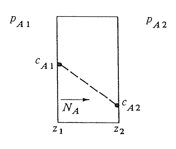
Mass transport in liquid – example 1 EMCD
The equimolar counter diffusion (EMCD) case in liquid also satisfies \(N_A + N_B = 0\)
From notes in Lecture 2, we can directly write the solution for \(N_A\):
\[ N_A = \frac{D_{AB}}{z_2 - z_1} (c_{A1} - c_{A2}) \]
Often for dilute A solution, we can rewrite the EMCD solution using average concentration.
EMCD solution in liquid
\[\begin{align} \boxed{ N_A = \frac{D_{AB} c_{A, v}}{z_2 - z_1} (x_{A1} - x_{A2}) } \end{align}\]We define \(c_{av}\) as the average total concentration in A+B (not A alone!):
\[ c_{av} = \left(\frac{\rho}{M}\right) = \frac{1}{2} \left(\frac{\rho_1}{M_1} + \frac{\rho_2}{M_2}\right) \]
- \(\rho_1\) and \(\rho_2\) are average density of solution at points 1 and 2
- \(M_1\) and \(M_2\) are average molecular weight of the solution at points 1 and 2
- What is the assumption if we can use the average \(c_{av}\) in this case?
Example 2 stagnant \(B\) (\(N_B = 0\))
- EMCD in liquid is very rare, stagnant B case more frequent
- Typical setup: diffusion through liquid films, where liquid molecules cannot permeate the barrier
Recall gas-phase equation:
\[ N_A = \frac{D_{AB} \, p_T \, (p_{A1} - p_{A2})} {R T \, (z_2 - z_1) \, p_{B,m}} \]
We have similarly in liquid:
\[\begin{align} \boxed{ N_A = \frac{D_{AB}c_{A, v}}{(z_2 - z_1)} \frac{(x_{A1} - x_{A2})}{x_{B,m}} },\quad x_{B,m} = \frac{x_{B2} - x_{B1}}{\ln\!(x_{B2} / x_{B1})} \end{align}\]Stagnant \(B\): further discussions
- \(x_{B,m}\) is the log-mean value of \(x_B\)
- In diluted A through stagnant B, we often have \(x_{B1} \approx x_{B2} \approx 1\)
- A simpler approximation can be made \(x_{B,m} \approx \frac{x_{B1} + x_{B2}}{2}\)
- We can even roughly approximate \(x_{B, m} = 1\)!
Diffusivity in liquid
Experimentally measured \(D_{AB}\) in liquid:
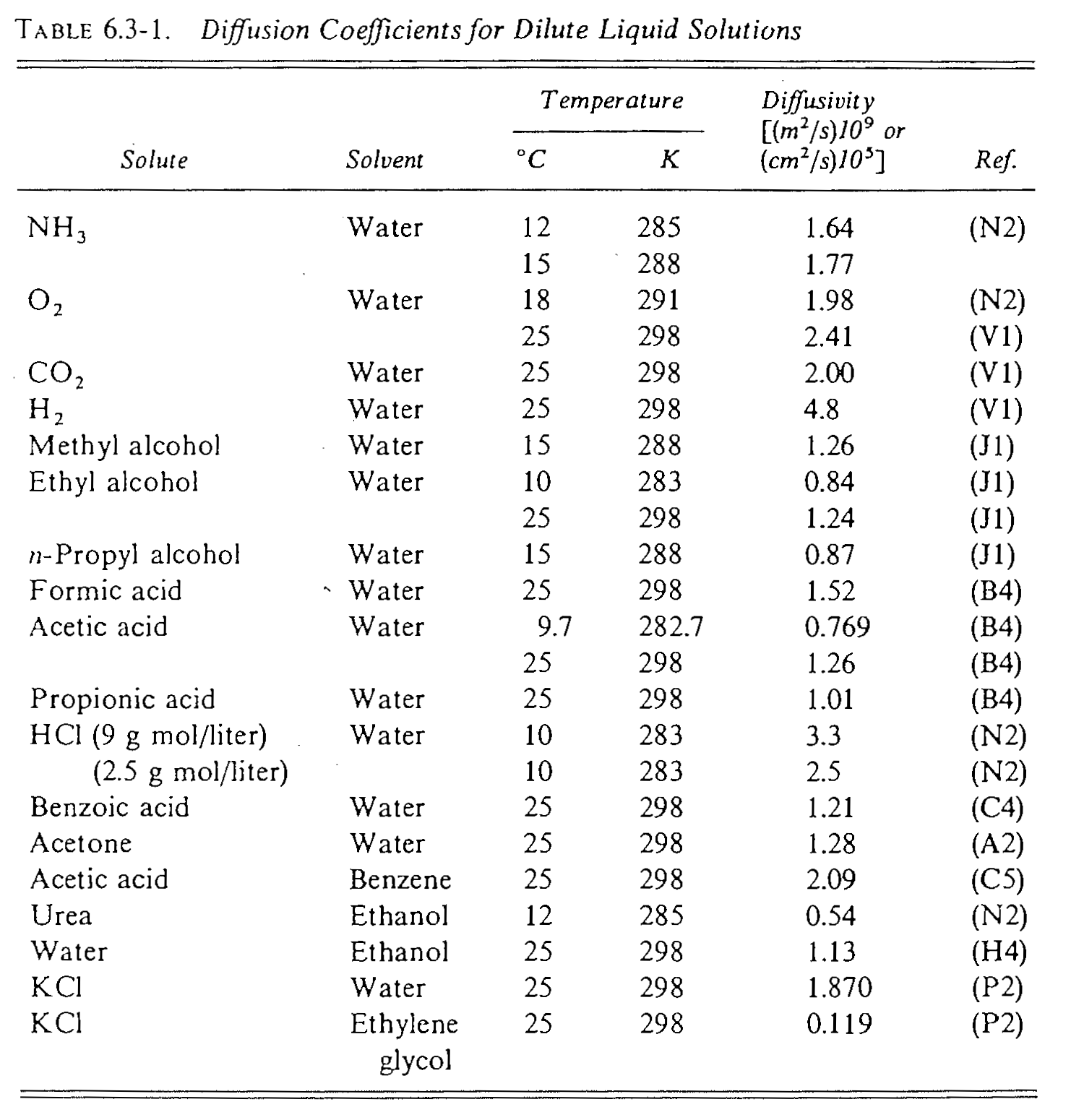
Prediction of diffusivity in liquid
- Molecular diffusion in liquid encounters much more collision than gas phase!
- Kinetic theory is not applicable!
- A few semi-empirical laws exist:
Einstein-Stokes Equation
- Model molecules A as spheres through a fluid B
- Drag force of A in B predicted from Stoke’s law
\[ D_{AB} = \mu_{AB} k_B T \]
where \(\mu_{AB}\) is the mobility of A in B
Einstein-Stokes equation for \(D_{AB}\)
Stokes–Einstein correlation for diffusivity in liquids:
\[ D_{AB} = \frac{9.96 \times 10^{-16}\, T} {\eta \, V_A^{0.333}} \]
- \(D_{AB}\) in \(\mathrm{m^2/s}\)
- \(T\) : temperature (K)
- \(\eta_B\) : viscosity of B (kg / m·s)
- \(V_A\) : molar volume of solute \(A\)
- evaluated at normal boiling point
- units: m\(^3\)/kg mol
- evaluated at normal boiling point
- ✔ Good for:
- Molecular weight \(> 1000\)
- \(V_A > 0.5\) m\(^3\)/kg mol
- ✘ Poor accuracy otherwise
Semi-empirical Wilke–Chang equation for liquids
\[ D_{AB} = \frac{1.173 \times 10^{-16}\, (\phi M_B)^{1/2}\, T} {\eta_B \, V_A^{0.6}} \]
- \(D_{AB}\) in \(\mathrm{m^2/s}\)
- \(T\) : temperature (K)
- \(\eta_B\) : viscosity of solvent \(B\) (kg / m·s)
- \(M_B\) : molecular weight of solvent \(B\)
- \(V_A\) : molar volume of solute \(A\) (m\(^3\)/kgmol)
- \(\phi\) : solvent association parameter (see next slide)
- Typical error:
- 10–15% for aqueous systems
- ~25% for non-aqueous solvents
- Valid temperature range:
- \(278\ \text{K} < T < 313\ \text{K}\)
Wilke–Chang equation, \(\phi\) values
Association parameter \(\phi\)
- Water: \(\phi = 2.6\)
- Methanol: \(\phi = 1.9\)
- Ethanol: \(\phi = 1.5\)
- Benzene: \(\phi = 1.0\)
- Non-associating solvents: \(\phi \approx 1.0\)
Diffusion in solids
- Slowest mode of mass transfer
- Vital to industry:
- Packaging
- Catalysts
- Biological processes
- We will focus on two types of solids
Type 1: homogeneous solids
- Uniform solid matrix
- Diffusion follows Fick’s law
- Well-defined diffusion path
Examples
- \(O_2\) diffusion through plastic
- \(H_2O\) diffusion through paint
Type 1: general flux equation for solids
For diffusion of \(A\) in a homogeneous solid:
\[ N_A = - c_T D_{AB} \frac{d x_A}{d z} + x_A (N_A + N_B) \]
In solids:
- Solid matrix is stationary
- \(v_m = 0 \;\Rightarrow\; (N_A + N_B) = 0\)
\[ \boxed{ N_A = - c_T D_{AB} \frac{d x_A}{d z} } \]
Final flux expression (concentration form)
Key properties for diffusion in solids:
- \(D_{AB}\) is independent of pressure
- \(D_{AB} \neq D_{BA}\)
For steady-state diffusion through a slab:
\[ \boxed{ N_A = \frac{D_{AB}\,(c_{A1} - c_{A2})} {(z_2 - z_1)} } \]
Assumptions:
- Slab geometry
- Homogeneous solid matrix
- Constant \(D_{AB}\)
How do we know \(c_{A}\)?
For this type of problem, we are often interested in the gas solubility in solid, where \(c_A \propto p_{A}\). When expressed using the solubility \(S\) :
\[ \boxed{ c_A = \frac{S\, p_A}{22.414} } \]
Unit:
- \(c_A\): \(\text{kg mol}\cdot\text{m}^{-3}\)
- \(S\): \(\text{m}^3\) (STP at 0 ℃ and 1 atm)
- \(p_A\): atm
Often we also express the permeability of a gas (\(P_{M}\)) in solid using \(P_M = S D_{AB}\)
Type 2: inhomogeneous solids
- Non-uniform structure
- Diffusion through:
- Pores
- Fixed or tortuous paths in solid matrix
- Requires modified Fick’s law
Examples:
- Brita water filter
- Porous catalysts
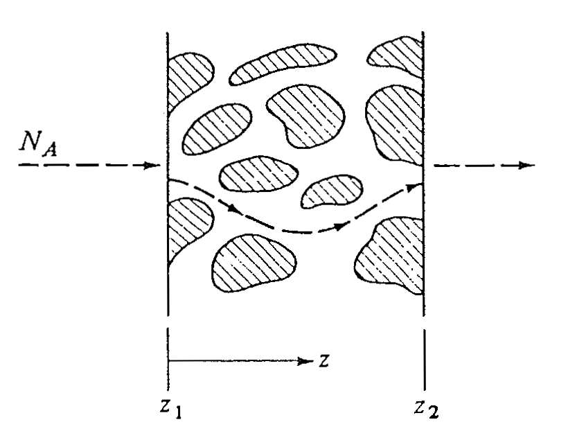
Flux in porous solids
Steady-state diffusion of \(A\) through a porous solid:
\[ N_A = \frac{\varepsilon}{\tau} \frac{D_{AB}\,(c_{A1} - c_{A2})} {(z_2 - z_1)} \]
- \(\varepsilon\): open void fraction
- typically 0.1–0.9
- \(\tau\): tortuosity
- typically 1.5–5 for solids
Effective diffusivity
Porous-media effects are lumped into an effective diffusivity:
\[ \boxed{ D_{AB,\text{eff}} = \frac{\varepsilon}{\tau}\, D_{AB} } \]
- Accounts for reduced area and increased path length
- Used directly in Fick’s law for porous solids
Example Problems
General steps
See handwritten notes for step-by-step solutions.
- Draw the physical scheme
- Identify the diffusion case
- List assumptions
- Write the governing flux equation
- Apply boundary conditions (optional)
- Solve for the molar flux
Example 1: EMCD basics
Adapted from Geankoplis 6.2-1
Ammonia (\(A\)) is diffusing through nitrogen (\(B\)) in a straight tube of length \(L = 0.10\) m at steady state.
The system is maintained at a total pressure of \(P_T = 1.0132 \times 10^5\) Pa and a temperature of \(T = 298\) K.
The partial pressure of ammonia at \(z_1\) is \(p_{A1} = 1.013 \times 10^4\) Pa, and at \(z_2\) is \(p_{A2} = 0.507 \times 10^4\) Pa.
The binary diffusivity of ammonia in nitrogen is \(D_{AB} = 0.230 \times 10^{-4}\) m\(^2\)/s.
- Determine values for fluxes of A and B.
Example 2: EMCD in two-bulb setup
Two bulbs with \(V_1=V_2\) are connected by a narrow tube of length \(L=0.15\) m and diameter \(d=1\) mm. The system is at \(T=25\ ^\circ\)C and \(P=1\) atm. Species \(A\) is \(N_2\) and species \(B\) is \(H_2\), with \(D_{AB}=0.784\) cm\(^2\)/s.
At \(t=0\):
- Left bulb: \(x_{N_2}=1.00\), \(x_{H_2}=0.00\)
- Right bulb: \(x_{N_2}=0.00\), \(x_{H_2}=1.00\)
At time \(t=t_1\):
- Left bulb: \(x_{N_2}=0.80\)
- Right bulb: \(x_{N_2}=0.25\)
- Determine the molar fluxes \(N_A\) and \(N_B\) at \(t=t_1\) (include direction).
- Find the value for \(v_{Ad}\) (diffusive velocity)
Example 3: diffusion through stagnant B with changing path length
Adapted from Geankoplis 6.2-3
Water vapor diffuses through a stagnant gas in a narrow vertical tube, dry air is constantly blown at the top of tube.
At time \(t\), the liquid level is a distance \(z\) from the tube top (i.e., the diffusion path length is \(z\)).
As diffusion proceeds, the liquid level drops slowly, so \(z\) increases with time.
- Derive an expression for the time \(t_F\) required for the level to drop such that the diffusion path length changes from \(z=z_0\) at \(t=0\) to \(z=z_F\) at \(t=t_F\).
Hint: use pseudo steady-state assumption
Example 4: determine \(D_{AB}\) through evaporation
Adapted from Griskey 10-2
Sample setup as example 4, a vertical tube of diameter \(D=0.01128\) m contains a liquid volatile species \(A\) (chloropicrin, \(CCl_3NO_2\)) evaporating into stagnant air (\(B\)) at 1 atm. The gas-phase diffusion of \(A\) occurs through the air column above the liquid surface.
At \(t=0\), the distance from the tube top to the liquid surface is \(z_0 = 0.0388\) m, after \(t=1\) day, the distance is \(z_1 = 0.0412\) m.
- Vapor pressure at the interface: \(p_{A1} = 3178.3\) Pa
- Liquid density: \(\rho_A = 1650\) kg/m\(^3\)
- Molecular weight: \(M_A = 164.39\) kg/kmol
- Use your expression from example 3, determine the binary diffusivity \(D_{AB}\) of \(A\) in air.
Summary
- Compare diffusion in gas and in liquid
- \(D_{AB}\vert_{l} \ll D_{AB}\vert_{g} \\ D_{AB}\vert_{s}\)
- Theories for predicting diffusivity in liquid, and when to apply them