CHE 318 Lecture 03
Molecular Diffusion in Gases: General Solutions
- Slides 👉 Open presentation🗒️
- PDF version of course note 👉 Open in pdf
- Handwritten notes 👉 Open in pdf
Recap
- Governing equation for diffusion binary mixture gas systems \[ N_{A} = -c_T D_{AB} \dfrac{d x_A}{dz} + x_A(N_A + N_B) \]
- Case 1: equimolar counter diffusion (EMCD)
- \(N_A + N_B = 0\)
- \(N_A = -c_T D_{AB} \dfrac{d x_A}{d z}\)
- Linear \(x_A\), \(c_A\) and \(p_A\) profiles
- \(N_A = \dfrac{D_{AB}}{RT(z_2 - z_1)}(p_{A1} - p_{A2})\)
- Case 2: diffusion through stagnant B
- \(N_B = 0\)
- \(N_A(1 - x_A) = -c_T D_{AB}\dfrac{d x_A}{dz}\)
- Usually in log-mean pressure form
- \(N_A = \dfrac{D_{AB}}{RT(z_2-z_1)} \dfrac{p_T}{p_{Bm}} \left(p_{A1} - p_{A2}\right)\)
Office hour
- Wednesday 11:15 - 12:15
- DICE 12-245
- Can take place in other meeting rooms if many people are attending
- Please use seminar time wisely for assignment questions!
Learning outcomes
After this lecture, you will be able to:
- Recall the conditions associated with common binary gas-transport cases.
- Describe the general solution for mass transport in a binary gas mixture.
- Formulate governing equations for common binary-diffusion systems.
- Apply the general solution to flux and composition calculations.
- Analyze pressure and concentration profiles predicted by the model.
Deriving the general solution (I)
General case for steady state (S.S) transport
- \(N_B = k N_A\) (\(k\) is a constant. why?)
- Only \(x_A\) (or \(c_A\), \(p_A\)) dependent on \(z\), not \(N_A\) or \(N_B\) 👉 separation of variables!
Deriving the general solution (II)
- L.H.S.
\[ \int_{z_1}^{z_2} \frac{dz}{D_{AB} c_T} = \frac{(z_2 - z_1)}{D_{AB} c_T} \]
- R.H.S.
Using substitution \(u = N_A - x_A (N_A + N_B)\), \(d u = -(N_A + N_B)\,dx_A\)
\[\begin{align} \int_{x_{A1}}^{x_{A2}} -\dfrac{dx_A}{N_A - x_A (N_A + N_B)} &= - \cdot - \frac{1}{N_A + N_B} \ln\!\left[N_A - x_A (N_A + N_B)\right] \bigg\vert_{x_{A1}}^{x_{A2}} \\ &= \frac{1}{N_A + N_B} \ln\!\left[\dfrac{ N_A - x_{A2} (N_A + N_B)} {N_A - x_{A1} (N_A + N_B)} \right] \end{align}\]Deriving the general solution (III)
We want to solve for \(N_A\)
\[\begin{align} \frac{(z_2 - z_1)}{c_T D_{AB}} &= \frac{1}{N_A + N_B} \ln\!\left[\dfrac{ N_A - x_{A2} (N_A + N_B)} {N_A - x_{A1} (N_A + N_B)} \right] \\ N_A &= \frac{c_T D_{AB}}{(z_2 - z_1)} \frac{N_A}{N_A + N_B} \ln\!\left[\dfrac{ N_A - x_{A2} (N_A + N_B)} {N_A - x_{A1} (N_A + N_B)} \right] \end{align}\]We can gather all \(N_A / (N_A + N_B)\) in the R.H.S since it’s a constant
\[\begin{align} \boxed{ N_A = \frac{ c_T D_{AB}}{(z_2 - z_1)} \left(\frac{N_A}{N_A + N_B}\right) \% \ln\!\left[ \dfrac{\frac{N_A}{N_A + N_B} - x_{A2}} {\frac{N_A}{N_A + N_B} - x_{A1}} \right] } \end{align}\]- This is the general solution for binary gas transport.
- Also works for \(N_A = -N_B\) (EMCD), with a little bit trick
Relation between gen. sol. and EMCD
The general solution is not applicable \(N_B = -N_A\), but we can prove \(N_B / N_A \to -1\) reduces to the EMCD equation.
- Let \(s = N_A / (N_A + N_B)\), so \(s \to \infty\) when \(N_B/N_A \to -1\)
- Use the Taylor expansion that \(\lim_{u \to 0} \ln(1-u) = -u\)
This is the EMCD result!
Three forms of gass mass transport equations (I)
In \(c_A\) form
- Case 1: EMCD
- \(N_A + N_B = 0\) \[ N_A = \dfrac{D_{AB}}{(z_2 - z_1)}(c_{A1} - c_{A2}) \]
- Case 2: stagnant B
- \(N_B = 0\)
General solution
- \(N_B = k N_A\)
\[ N_A = \frac{D_{AB} c_T}{(z_2 - z_1)} \frac{N_A}{N_A + N_B} \ln\!\left[\dfrac{ \frac{N_A}{N_A + N_B} - \frac{c_{A2}}{c_T}} {\frac{N_A}{N_A + N_B} - \frac{c_{A1}}{c_T}} \right] \]
Three forms of gass mass transport equations (II)
In \(x_A\) form
- Case 1: EMCD
- \(N_A + N_B = 0\) \[ N_A = \dfrac{D_{AB} c_T}{(z_2 - z_1)}(x_{A1} - x_{A2}) \]
- Case 2: stagnant B
- \(N_B = 0\)
General solution
- \(N_B = \lambda N_A\)
\[ N_A = \frac{D_{AB} c_T}{(z_2 - z_1)} \frac{N_A}{N_A + N_B} \ln\!\left[\dfrac{ \frac{N_A}{N_A + N_B} - x_{A2}} {\frac{N_A}{N_A + N_B} - x_{A1}} \right] \]
Three forms of gass mass transport equations (III)
In \(p_A\) form (ideal gas)
- Case 1: EMCD
- \(N_A + N_B = 0\) \[ N_A = \dfrac{D_{AB}}{RT(z_2 - z_1)}(p_{A1} - p_{A2}) \]
- Case 2: stagnant B
- \(N_B = 0\)
General solution
- \(N_B = \lambda N_A\)
\[ N_A = \frac{D_{AB} p_T}{RT(z_2 - z_1)} \frac{N_A}{N_A + N_B} \ln\!\left[\dfrac{ \frac{N_A}{N_A + N_B} - x_{A2}} {\frac{N_A}{N_A + N_B} - x_{A1}} \right] \]
General solution – \(x_A(z)\) profile
In all the cases we study the S.S. condition:
\[\frac{d N_A}{d z} = 0\]
For the general case \(s = N_A / (N_A + N_B)\), we have
\[\begin{align} \frac{dN_A}{dz} &= \frac{d}{dz} \left[ \frac{D_{AB} c_T}{s - x_A} \frac{d x_A}{d z}\right] = 0\\ \frac{D_{AB} c_T}{s - x_A} \frac{d x_A}{d z} &= \mathrm{Const} \end{align}\]\(x_A(z)\) has a general solution with exponential form (with \(K_1\) and \(K_2\) being constants)
\[\begin{align} \boxed{ x_{A} = s - K_1 e^{K_2 z} } \end{align}\]\(x_A(z)\) profile
Notes on the relation between \(N_A\) and \(N_B\) (1)
Using steady state condition, we need to know relation between \(N_A\) and \(N_B\) before solving the general EQ.
It depends on the system setup and mass balance.
Let’s consider the same chemical reaction of hydrogen dissociation by a solid catalst
\[\begin{align} \text{H}_2\ (A, \text{gas}) \rightarrow 2\text{H}^*\ (B, \text{gas}) \end{align}\]Case 1: reaction through a solid catalyst at bottom of a tube
- The flux of A and B have opposite signs
- \(N_B = -2 N_A\)
Notes on the relation between \(N_A\) and \(N_B\) (2)
Case 2: gas flow through a solid catalyst inside a tube
- The flux of A and B have the same sign
- \(N_B = 2 N_A\)
Take home question: - How do the flux directions affect the general solution?
Measuring diffusivity \(D_{AB}\) in gases
- Several experimental methods exist for gases, evaporated liquid and sublimated solids (see Geankoplis Ch 6.2E)
- We will introduce the two-bulb method for gases
- Typical setup see Duncan & Toor AIChE J. 1962, 8, 38-41
- Which case should we apply?
Two-bulb experiment: conditions
Conditions for the two-bulb experiment
- Initially, pure A in bulb 1 and pure B and bulb 2
- \(t=0\), the valve is opened slowly to minimize convection
- \(t=t_e\), the valve is closed and the composition in 1 and 2 are analyzed
- The valve open time is much shorter than \(t_2 - t_1\)
- The tube is a very thin capillary 👉 no convection
- Constant \(p_T\) and \(T\) throughout experiment
Two-bulb experiment: pseudo steady state
We can apply:
- EMCD condition (no convection)
- Pseudo-steady state (P.S.S) assumption
- At each time step, we assume \(N_A\) or \(J_{Az}^*\) is constant (linear \(c_A\) profile)
- But net \(N_A\) flux accumulates A molecules in bulb 2
- \(c_A\) in bulb 2 changes over time
Two-bulb experiment: governing equations
We use the mass balance of the system
\[\begin{align*} \text{[Mass In]} &= \text{[Accumulation]} \\ S \cdot J_{Az}^* &= V_2 \frac{d c_{A2}}{dt} \\ D_{AB} \frac{c_{A1} - c_{A2}}{L} \cdot S &= V_2 \frac{d c_{A2}}{dt} \end{align*}\]Since the total pressure \(p_T\) is constant, the average concentration of \(c_A\) in the system, \(c_{A, av}\) is also constant
\[\begin{align*} V_T c_{A, av} &= (V_1 + V_2)c_{A, av} \\ &= V_1c_{A1}(t=0) + V_2c_{A2}(t=0) \\ &= V_1c_{A1}(t\neq0) + V_2c_{A2}(t\neq0) \end{align*}\]Two-bulb experiment: solutions
We are interested in \(c_{A2}\), so substitute \(c_{A1}\) with relation to \(c_{A, av}\):
\[ c_{A1} = \frac{V_T c_{A, av} - V_2 c_{A2}}{V_1} \]
After the substitution, rearrangement and integration we get:
\[\begin{align*} \ln\!\left[ \frac{c_{A, av} - c_{A2}(t=t_e)}{c_{A, av} - c_{A2}(t=0)} \right] &= -\frac{D_{AB} V_T S}{V_1 V_2 L} \cdot t \\ \end{align*}\]We can extract \(D_{AB}\) using the slope of the plot!
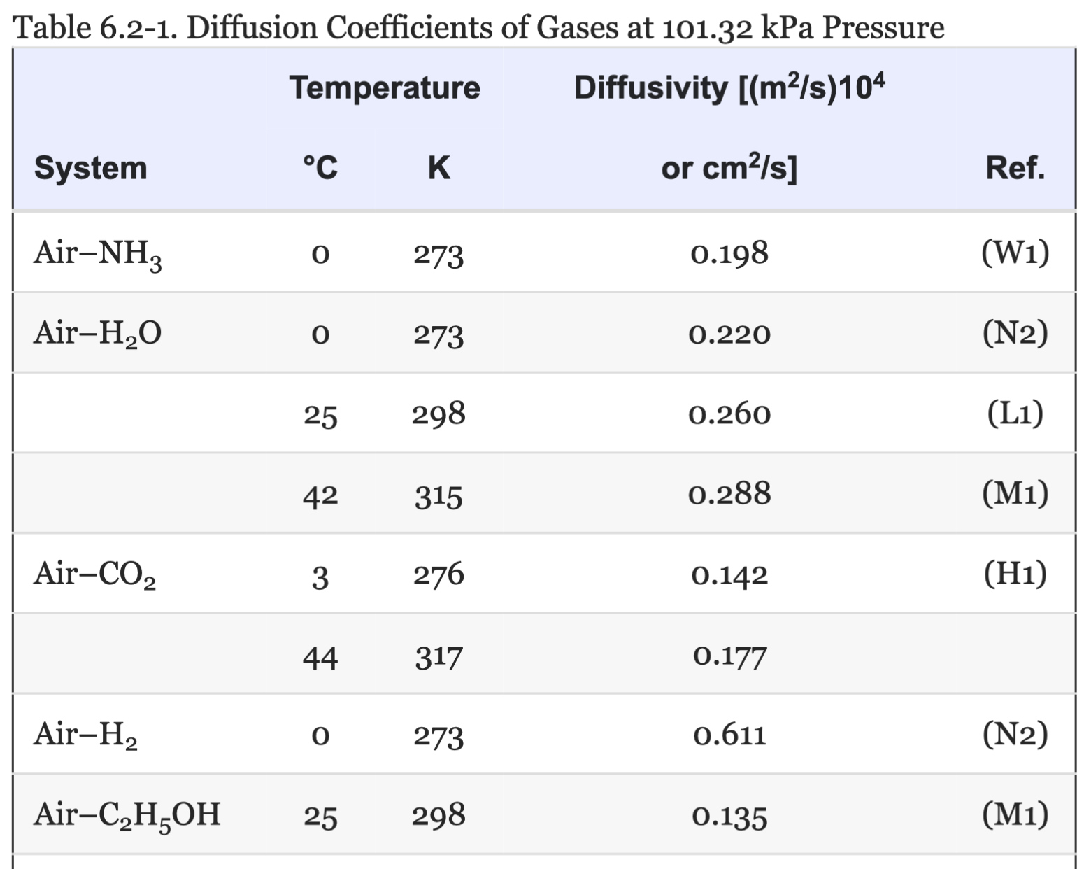
Some typical diffusivity measurements
Summary
- General solutions for \(N_B = k N_A\) extend the earlier EMCD and stagnant-B cases.
- The resulting flux expression takes a logarithmic form, similar to the stagnant-B solution.
- Once boundary compositions are known, the flux is controlled by the relation between \(N_A\) and \(N_B\).
- The two-bulb experiment provides a practical way to determine gas diffusivity.
Preview of next class: theories for predicting \(D_{AB}\)
- Kinetic theory
\[ D_{AB} = \frac{1}{3} \overline{u} \lambda \]
- Chapman-Enskog theory
\[ D_{AB} \propto \frac{T^{\frac{3}{2}}}{P} \left(\frac{1}{m_A} + \frac{1}{m_B} \right)^{\frac{1}{2}} \]
- Fuller method
\[ D_{AB} \propto \frac{T^{1.75}}{P} \left(\frac{1}{m_A} + \frac{1}{m_B} \right)^{\frac{1}{2}} \]
Footnotes
Geankoplis Table 6.2-1↩︎