CHE 318 Lecture 06
Steady State Mass Transfer – Other Geometries
- Slides 👉 Open presentation🗒️
- PDF version of course note 👉 Open in pdf
- Handwritten notes 👉 Open in pdf
Recap
- Diffusion in liquid and solid
- Much slower than gas (\(D_{AB}\) orders of magnitudes smaller)
- Theories to predict \(D_{AB}\) in liquid (Stokes-Einstein, Wilke-Chang)
- Effective diffusivity in solid (void fraction ε; tortuosity τ)
- Solving \(N_A\) in liquid
- EMCD: rare case
- Stagnant B: approximating \(x_{Bm}\)
- Calculating \(c_{av}\) concentration
- Solving \(N_A\) in solid (thin membrane permeability)
- Use of solubility \(S\)
- Permeability \(P_{M} = S D_{AB}\)
Learning outcomes
After this lecture, you will be able to:
- Recall how diffusion equations change across planar, cylindrical, and spherical geometries.
- Describe approximations used to simplify expressions for \(N_A\).
- Identify when the stagnant-B framework is appropriate for spherical-diffusion problems.
- Apply pseudo-steady-state analysis to diffusion problems in variable-area systems.
- Calculate diffusivities from evaporation-based experiments.
Examples for Diffusion in Liquid and Solid
Example 1: gas diffusion through liquid film
Adapted from Geankoplis Problem 6.3-2
Diffusion of Ammonia in an Aqueous Solution. An ammonia (A)–water (B) solution at 278 K and 4.0 mm thick is in contact at one surface with an organic liquid at this interface. The concentration of ammonia in the organic phase is held constant and is such that the equilibrium concentration of ammonia in the water at this surface is 2.0 wt % ammonia (density of aqueous solution 991.7 kg/m3) and the concentration of ammonia in water at the other end of the film 4.0 mm away is 10 wt % (density 961.7 kg/m3). Water and the organic are insoluble in each other. The diffusion coefficient of NH3 in water is \(1.24\times{}10^{−9}\) m\(^2\)/s.
- At steady state, calculate the flux \(N_A\) in kg mol/s·m\(^2\)
- Calculate the flux \(N_B\). Explain.
Example 1: solutions
See handwritten notes for step-by-step solutions.
- Determine the type of system if water-organic layer is inpenetratable (answer question b first)
- Refere to Lecture 1 for conversion between wt%, molar fraction and concentration.
Answer:
- \(N_A = 1.52\times{}10^{6}\ \text{kg mol}\cdot\text{m}^{-2}\cdot\text{s}^{-1}\)
- \(N_B=0\) (diffusion through stagnant film)
Example 2: diffusion through solid film (solubility)
Adapted from Geankoplis Problem 6.5-1
A flat plug 30 mm thick having an area of \(4.0\times10^{−4}\ \text{m}^2\) and made of vulcanized rubber is used for closing an opening in a container. The gas CO2 at 25 °C and 2.0 atm pressure is inside the container. Calculate the total leakage or diffusion of CO2 through the plug to the outside in kg mol CO2/s at steady state. Assume that the partial pressure of CO2 outside is zero. From Barrer (B5) the solubility of the CO2 gas is 0.90 \(m^3\) gas (at STP of 0°C and 1 atm) per m3 rubber per atm pressure of CO2. The diffusivity is \(0.11\times{}10^{−9}\) m\(^2\)/s.
Example 2: solution
- Notice the unit for symbols when applying \(c_A = S P_A / (22.414)\)
- What unit should total leakage have?
Answer:
- Total leakage rate \(1.178\times{}10^{-13}\ \text{kg mol}\cdot\text{s}^{-1}\)
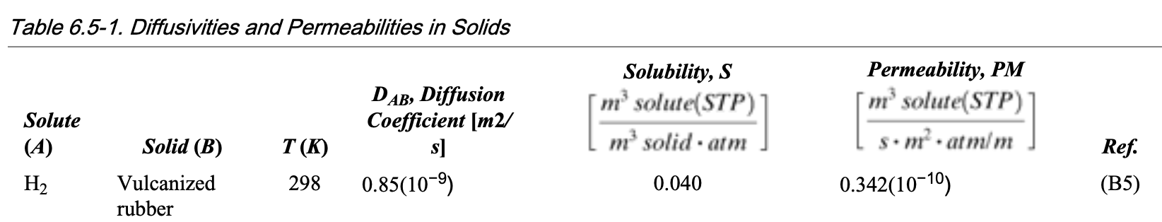
Example 3: use of permeability
Adapted from Geankoplis Problem 6.5-3
The gas hydrogen is diffusing through a sheet of vulcanized rubber 20 mm thick at 25 °C. The partial pressure of H2 is 1.5 atm inside and 0 outside. Using the data from Table 6.5-1 (see below), calculate the following:
- The diffusivity \(D_{AB}\) from the permeability \(P_M\) and solubility \(S\), and compare with the value in the table.
- The flux \(N_A\) of H2 at steady state.
Example 3: solution
Answer:
- Use \(D_{AB} = P_M / S\) (note the unit)
- \(N_A = 1.144\times{}10^{-10}\ \text{kg mol}\cdot\text{m}^{-2}\cdot\text{s}^{-1}\)
Solving Diffusion Through Varying Area
Diffusion through varying cross-sectional area
Steady state mass balance
Many industrial applications involde 1D transport with variable area \(A(z)\), with mass balance:
\[\begin{align} [\mathrm{In}] - [\mathrm{Out}] &= 0 \\ N_{A1} A_1 - N_{A2} A_2 &= 0 \end{align}\]Define the total molar flow rate of A:
\[ \overline{N}_A = N_A \, A(z) \]
At steady state: - \(\overline{N}_A\) is constant - \(N_A\) varies with position if \(A(z)\) (or \(A(r)\)) varies
Applications of variable-area diffusion
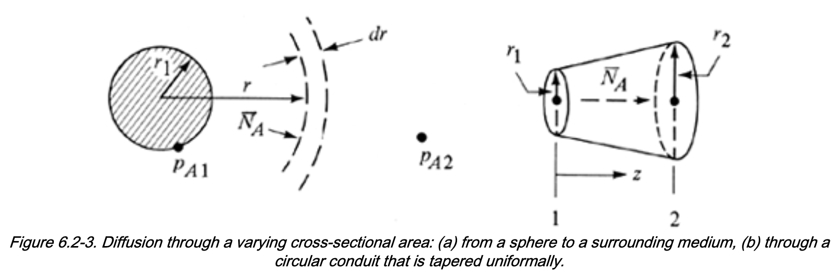
This framework can be used to solve diffusion through:
- Sphere
- Cylinder
- Tube with varying diameter
- Any system with a known area function \(A = A(z)\) or \(A=A(r)\)
Key ideas
- Do not solve as simple 1D Cartesian diffusion
- Geometry enters through \(A(z)\)
- Flux adjusts to maintain constant \(\overline{N}_A\)
Summary
- Solving various examples in liquid and gas diffusion systems
- Use of weight %, log-mean molar ratio, solubility and permeability