CHE 318 Lecture 14
Mass Transfer Coefficients (II)
- Slides 👉 Open presentation🗒️
- PDF version of course note 👉 Open in pdf
- Handwritten notes 👉 Open in pdf
Recap
- Introduction to mass transfer coefficients
- Link between mass transfer coefficient and diffusivity
- Introduction to boundary concentration problem
Learning outcomes
After this lecture, you will be able to:
- Recall flux equations written with mass transfer coefficients in different phases.
- Describe why coefficient-based descriptions are useful for interfacial transport.
- Identify the units and meanings of common mass transfer coefficients.
- Apply conversions between coefficient forms used in gas- and liquid-phase analyses.
Realistic interfacial concentration profiles
At the boundary, it is often convenient to use the equilibrium concentration ratio between gas (\(c_i\)) and liquid (\(c_{Li}\)). This constant, often called the equilibrium distribution coefficient, is defined as:
\[\begin{align} K &= \frac{\text{[Conc. at gas side]}}{\text{[Conc. at liquid side]}} \\ &= \frac{c_{i}}{c_{Li}} \end{align}\]- Similarity: Henry’s law (\(H = \dfrac{p_{\text{gas}}}{c_{\text{aq}}}\)), remember in gas \(p_{\text{gas}} = c_{\text{gas}} RT\)
- We have already seen similar concepts in solubility in liquid / solid diffusion equations!
- \(K\) can be a value range from \(0\) to \(\infty\) 👉 what does that mean?
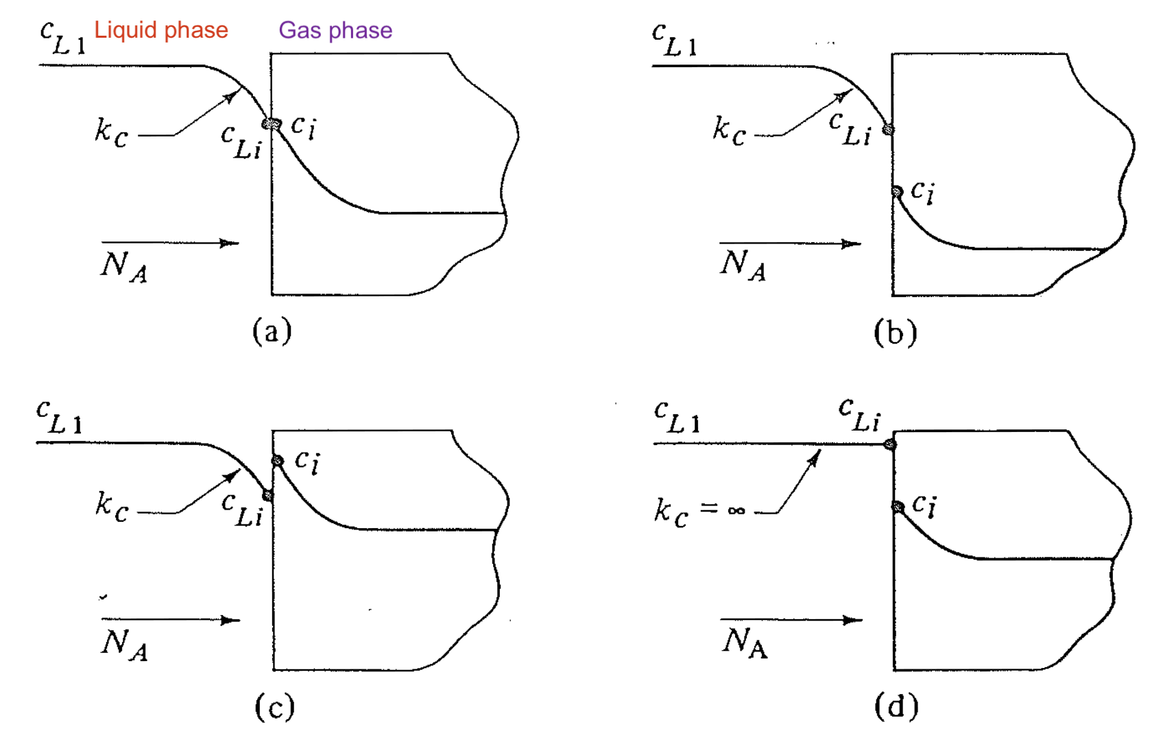
Interfacial concentration profile for different \(K\)
- The interfacial concentration values depend on the value of \(K\)!
- What else determines the interfacial balance? 👉 matching of interfacial fluxes \(N_A\) at both sides!
Match of interfacial fluxes
At equilibrium, if there is no resistance when transferring A between the interface, what is the mass balance equation?
\[\begin{align} \text{[In]}\vert_{\text{left}} - \text{[Out]}\vert_{\text{right}} + \text{[Gen]}\vert_{\text{interface}} &= \text{[Acc]}\vert_{\text{interface}} \\ N_A\vert_{\text{left}} = N_A\vert_{\text{right}} \end{align}\]How do we model \(N_A\) in each phase?
- May be a combination of diffusion and convection
- Fluid velocity at interface may be turbulent (hard to model)
- In general we use the phenomenal relation \(\text{[Flux]} = \text{[Driving Force]} / \text{[Resistance]}\)
General flux equation for convective transport regime
- The driving force is the concentration difference “bulk concentration” and “interfacial concentration”
- The resistance is lumped into one coefficient \(k_c'\), mass transfer coefficient.
- \(k_c'\) is inversely related to the resistance.
- \(k_c'\) means driving force is concentration & convection term is EMCD-like
- The unit of \(k_c'\)? 👉 \(\text{m}\cdot\text{s}^{-1}\)
- \(k_c'\) can be \(\infty\)! 👉 No transfer resistance inside the bulk phase
Where does \(k_c'\) come from (I)?
Simplified view: transport resistance of A from bulk to the interface occurs inside an interfacial film with thickness \(\delta\). We can write \(N_A\) at steady state using already known results
- Case 1: EMCD / diffusion-controlled / dilute transport in liquid
- Case 2: transport in stagnant film with non-negligible convection
- Can be written both by \(k_c'\) or \(k_c\) terms
- One can expect \(k_c\) contain the \(1/x_{Bm}\) term!
Where does \(k_c\) come from (II)?
The mass transfer coefficient \(k_c\) is even valid for systems with effective \(D_{AB}\)!
- Case 3: mass transfer in porous solid materials
- Case 4: turbulent mass transfer
The turbulence in the fluid contributes to an additional term \(\epsilon_m\) in diffusion terms
\[\begin{align} N_A &= \boxed{\frac{D_{AB} + \epsilon_m}{\delta}} (c_{L, b} - c_{L, i}) \\ &= k_c' (c_{L, b} - c_{L, i}) \end{align}\]- \(\epsilon_m\) is the “Eddie diffusivity” (correction to \(D_{AB}\) due to turbulence)
- General case for \(\epsilon_m\) is non-trivial to solve!
Implications of mass transfer coefficient \(k_c'\)
- Really convenient to use!
- In reality, \(k_c'\) is not a physics-based quantity, it depends on system / condition
- \(k_c' \propto D_{AB}^n\) in realistic systems
- We will discuss about different theories that explains the relation between \(k_c'\) and \(D_{AB}\) (penetration theory, film theory, boundary theory) in coming weeks
Balance equations at interfaces
We now have 2 equations to determine the interfacial concentrations!
- Equilibrium concentration distribution
- Flux matching
We can solve \(c_{L, i}\) and \(c_{g, i}\) given information about:
- Bulk concentrations \(c_{L, b}\), \(c_{g, b}\)
- Equilibrium distribution coefficient \(K\)
- Mass transfer coefficients \(k_c\) in each phase
Demonstration of mixed boundary conditions
Mass transfer coefficient in different forms
When using \(k\) to express flux, we have the same form (Geankoplis Table 7.2.1)
- Flux equations for EMCD
- Flux equations for diffusion through stagnant B
But:
- \(k_c'\) and \(k_c\) are two different coefficients
- \(k_c'\), \(k_L'\), \(k_G'\) have different units
Naming convention and units
- Superscript: EMCD \(k'_{\text{driving force}}\); Convective / stagnant B \(k_{\text{driving force}}\)
| Phase / Driving force | Concentration \(c_A\) | Partial pressure \(p_A\) | Mole fraction (gas \(y_A\), liquid \(x_A\)) |
|---|---|---|---|
| Gas phase | \(k_c\), \(k_c'\) | \(k_G\), \(k_G'\) | \(k_y\), \(k_y'\) |
| Liquid phase | \(k_c\), \(k_c'\) | – | \(k_x\), \(k_x'\) |
| Liquid (alt. form) | \(k_L\), \(k_L'\) | – | – |
| Unit of \(k\) | \(\text{m}\cdot\text{s}^{-1}\) | \(\dfrac{\text{kg mol}}{\text{s} \cdot \text{m}^2 \cdot \text{Pa}}\) | \(\dfrac{\text{kg mol}}{\text{s} \cdot \text{m}^2 \cdot \text{mol frac}}\) |
Conversions between mass transfer coefficients
Gas phase
\[\begin{align} k_c' \, c_T &= k_c' \frac{p_T}{RT} = k_c \frac{p_{Bm}}{RT} \\ &= k_G' \, p_T = k_G \, p_{Bm} \\ &= k_y' = k_y \, y_{Bm} \\ &= k_c \, y_{Bm} \, c_T = k_G \, y_{Bm} \, p_T \end{align}\]- \(p\) : total pressure
- \(p_{Bm}\) : log-mean partial pressure of inert \(B\)
- \(y_{Bm}\) : log-mean mole fraction of \(B\)
- \(c_T = p_T/(RT)\)
Liquid phase
\[\begin{align} k_c' \, c &= k_L' \, c = k_L \, x_{Bm} \, c \\ &= k_L' \, \frac{\rho}{M} = k_x' = k_x \, x_{Bm} \end{align}\]- \(\rho\) : liquid density
- \(M\) : molecular weight
- \(x_{Bm}\) : log-mean mole fraction of solvent \(B\)
Summary
- Interfacial concentration profiles depend on equilibrium constraints and the relative resistance of each phase.
- Matching fluxes across the interface allows us to determine interfacial compositions.
- Mass transfer coefficients can be expressed in multiple forms, but their units and meanings must be tracked carefully.
What to learn next
The concept of mass transfer coefficient \(k\) is both beautiful and ugly.
- We gain the simplicity of expressing flux equations using simple formula,
- We lose physical understanding about its origin in many systems
In next lectures, we will see:
- How to use mass transfer coefficients for different phases (gas, liquid, solid)
- How convective fluid transport is expressed using coefficients
- How to perform mass transfer analysis based on transfer coefficients