MATE 664 Lecture 04
Introduction to Diffusion
- Slides 👉 Open presentation🗒️
- PDF version of course note 👉 Open in pdf
- Handwritten notes 👉 Open in pdf
Recap of Lecture 03
Key ideas from last lecture:
- Entropy flux and production
- Rewriting entropy production in flux and driving force terms
- Direct and coupling coefficients
- Analysis of several cross-coupling effects in material science
Learning outcomes
After this lecture, you will be able to:
- Identify driving forces and fluxes for diffusive mass transport
- Derive Fick’s first law from irreversible thermodynamics using chemical potential
- Estimate diffusivities in gases, liquids, and solids
- Explain the temperature dependence of diffusivity using Arrhenius-type relations
- Describe the thermodynamic origin of self-diffusion
Recap: driving forces in irreversible thermodynamics
entropy balance: \[ \frac{ds}{dt} = -\nabla \cdot \vec{J}_s + \dot{\sigma} \]
entropy flux: \[ \vec{J}_s = \sum_i \frac{\psi_i}{T}\vec{J}_i \]
entropy production: \[ T\dot{\sigma} = -\sum_i \vec{J}_i \cdot \nabla \psi_i \ge 0 \]
When do \(\dot{\sigma}\) diminish? Orthogonality of flux and driving force
We will show one example that has non-trivial solution to \(\dot{\sigma} = 0\)
- entropy production vanishes if: \[ \vec{J}_i \cdot \nabla \psi_i = 0 \]
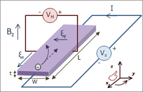
- Example: Hall effect
- Current flows while electric potential gradient is orthogonal
- Generalized for thermomagnetic and galvanomagnetic effects (Callen Phys. Rev. 1948, 73, 1349)
- Magnetic field induced symmetry breaking
- \(L_{ij}(H) = L_{ji}(-H)\)
Chemical potential as driving force
Consider one chemical species with chemical potential \(\mu\)
Definition: \[ \mu = \left(\frac{\partial U}{\partial N}\right)_{S,V} \]
\(\mu\) represents energy cost of adding more molecules
Diffusion driven by gradients in \(\mu\)
See analog to a water tank in handwritten notes
Entropy production and mass flux
Entropy production due to diffusion: \[ T\dot{\sigma} = -\vec{J}_m \cdot \nabla \mu \]
Linear law: \[ \vec{J}_m = -L_{MM}\nabla \mu \]
\(L_{MM}\): phenomenological mobility coefficient
From mobility to Fick’s law (determine \(L_{MM}\))
See analog in handwritten notes
Force balance and drift velocity (\(M\): mobility): \[ v = M \nabla \mu \]
Mass flux: \[ \vec{J} = c v = -M c \nabla \mu \]
Diffusion coefficient: \[ D = M k_B T \]
Chemical potential in mixtures
See analog in handwritten notes
For constant \(T,P\): \[ \mu_i = \left(\frac{\partial G}{\partial N_i}\right)_{T,P} \]
Chemical potential in a mixture solution: \[ \mu_i = \mu_i^0 + k_B T \ln \gamma_i x_i \]
activity coefficient \(\gamma_i = 1\) for ideal solution (Raoult’s law)
Fick’s first law
Substitute \(\mu_i\) into flux. For species \(i\) \[ \vec{J} = -D \nabla c \]
Assumptions:
- ideal solution
- constant \(T\)
- isotropic medium (\(D_{\alpha \beta}=D=\text{Const}\))
concentration gradient is a special case of \(\nabla \mu\)
What does diffusivity depend on?
- temperature
- concentration
- spatial position (??)
- general diffusion driven by \(\nabla \mu\)
- Fick’s law valid under restricted conditions
Fick’s second law
Mass conservation (no source term) \[ \frac{\partial c}{\partial t} = -\nabla \cdot \vec{J} \]
Substitution: \[ \frac{\partial c}{\partial t} = \nabla \cdot (D \nabla c) \]
If \(D_i\) is constant: \[ \frac{\partial c}{\partial t} = D_i \nabla^2 c \]
- \(\nabla^2\): Laplace operator
One-dimensional diffusion in isotropic homogeneous medium
1D equation: \[ \frac{\partial c}{\partial t} = D \frac{\partial^2 c}{\partial x^2} \]
Steady state: \[ \frac{\partial^2 c}{\partial x^2} = 0 \]
- Linear concentration profile!
Physical meaning of Laplace operator
\(\nabla^2 c\) measures curvature (sort of…)
Steady state implies zero curvature
Transient diffusion requires nonzero curvature
Curvature and Second Derivative
concave profile: \[ \frac{d^2 c}{dx^2} < 0 \]
convex profile: \[ \frac{d^2 c}{dx^2} > 0 \]
curvature determines smoothing direction
Typical magnitudes of diffusivity
- gases: \[ D \sim 10^{-5}\ \mathrm{m^2/s} \]
- liquids: \[ D < 10^{-9}\ \mathrm{m^2/s} \]
- solids: \[ D < 10^{-13}\ \mathrm{m^2/s} \]
Typical \(D\) range
A common misconception
Search for any youtube video with “diffusion experiment dye”
Can we verify whether the scenario seen is Ficknian diffusion?
Diffusion vs convection length scale
Length \(L\) traveled in time \(t\):
- Diffusion: \(L = 6\sqrt{D_{AB}\,t}\) (Einstein, ~1905)
- Convection: \(L = v_m\,t\)
What is typical \(D_{AB}\) in a liquid?
- Often \(D_{AB}\sim 10^{-9}\) to \(10^{-10}\,\mathrm{m^2/s}\)
Assuming \(D_{AB} = 10^{-10} \mathrm{m^2/s}\) \(v_{m} = 10^{-3} \mathrm{m/s}\)
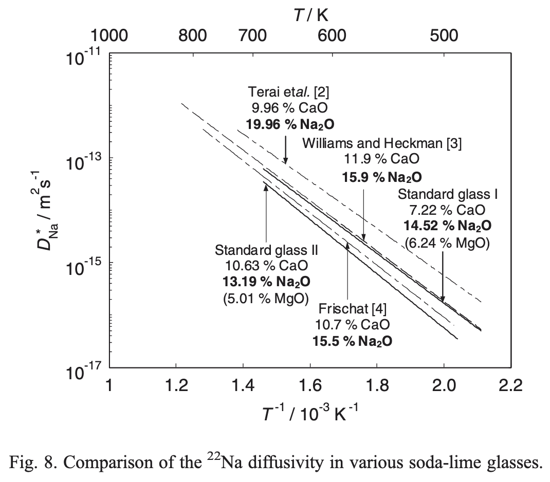
Temperature dependence of diffusivity
- Arrhenius form: \[ D = D_0 \exp\!\left(-\frac{\Delta H^a}{k_B T}\right) \]
- \(\Delta H^a\): activation enthalpy
- Why do we measure \(\Delta H_a\), not the \(\Delta G^a\)?
- How can you read the plot?
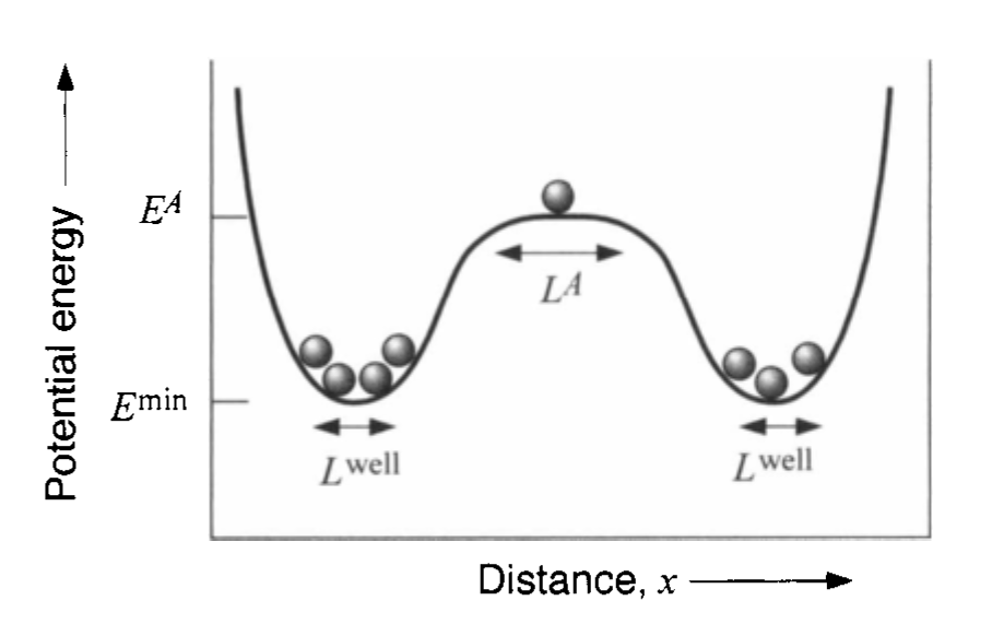
Physical interpretation of activation
- atoms hop between sites
- energy barrier must be overcome
- jump frequency: \[ \Gamma = \nu \exp\!\left(-\frac{\Delta G^\ddagger}{k_B T}\right) \]
- diffusion proportional to hop rate and distance
Multiple diffusion mechanisms
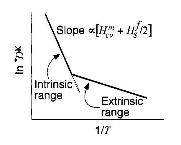
- Different diffusion paths
- Different activation energies
- Dominant mechanism controls slope of \(\ln D\) vs \(1/T\)
Diffusion in gases
Kinetic theory description
Chapman–Enskog result: \[ D \propto \frac{T^{3/2}}{P} \]
Collisions limit transport
Diffusion in liquids
Stokes–Einstein equation: \[ D = \frac{k_B T}{6\pi \eta r} \]
\(\eta\): viscosity
\(r\): particle radius
Is it accurate enough in polymer solutions?
Diffusion in solids
- Diffusion in solids is much more complex!
- Discrete lattice sites
- Mechanisms (non-exhaustive)
- Vacancy
- Ring mechanism
- Push-out mechanism
- Interstitial
- Strong temperature dependence
Vacancy diffusion mechanism
- Atoms exchange with vacancies
- Jump only if vacancy is adjacent
- Vacancy sources:
- Surfaces
- Grain boundaries
- Dislocations
Types of diffusivity
As the previous example of diffusion + convection video shows, the measurement of diffusivity really depends on which reference frame we use.
- Self-diffusivity \(D^*\)
- Intrinsic diffusivity \(D_i\) (lattice frame / C-frame; \(\mathtt{C}\) 👉crystal)
- Inter-diffusivity \(\tilde{D}\) (laboratory frame / V-frame; \(\mathtt{V}\) 👉volume-fixed)
Measuring self-diffusion
Isotope tracer experiments
Lattice constraint: \[ c_i + c_i^* + c_v = \text{const} \]
- General “network-constrained” problem
Vacancy concentration often at equilibrium
- Vacancy balance with the source (surface / grain boundary / dislocation)

Flux relations in network-constrained systems
- Flux driven by chemical potential differences (1D)
Non-radioactive species: \[ J_i = -L_{ii}\frac{\partial (\mu_i - \mu_v)}{\partial x} -L_{i{i}^*}\frac{\partial (\mu_{i^*} - \mu_v)}{\partial x} \]
Radioactive species: \[ J_{i^*} = -L_{{i^*}{i}}\frac{\partial (\mu_{i} - \mu_v)}{\partial x} -L_{{i^*}{i^*}}\frac{\partial (\mu_{i^*} - \mu_v)}{\partial x} \]
Vacancy (zero-flux, why?): \[ J_v = 0 \]
Vacancy equilibrium assumption
- \(\mu_v = \text{const}\)
- \(J_v = 0\)
- total flux balance: \[ J_i + J_i^* + J_v = 0 \]
Resulting self-diffusion flux
- Chemical potential gradient: \[ \frac{\partial \mu_{i^*}}{\partial x} = k_B T \frac{1}{c_i}\frac{\partial c_i}{\partial x} \]
- Self-diffusion coefficient: \[ D^{*} = k_B T\left(\frac{L_{ii}}{c_i} + \frac{L_{ii^*}}{c_{i^*}}\right) \]
Why self-diffusion occurs
- No macroscopic concentration gradient!
- Chemical potential varies locally
- Random walk lowers free energy
- Entropy maximization drives motion
Summary
- Diffusion is driven by chemical potential gradients
- Fick’s laws follow from irreversible thermodynamics
- Laplace operator reflects curvature and smoothing
- Diffusivity varies strongly with phase and temperature
- Self-diffusion exists even in homogeneous systems
Footnotes
Solid. State Ionics 2006, 177, 2839↩︎