MATE 664 Lecture 06
Solution to Diffusion Equations (I)
- Slides 👉 Open presentation🗒️
- PDF version of course note 👉 Open in pdf
- Handwritten notes 👉 Open in pdf
Recap of Lecture 05
Key ideas from last lecture:
- Different forms of diffusivities
- Deriving diffusivity from driving force terms
- Differentiate reference frames used for diffusion equations
Recap: intrinsic diffusivity expression
For component \(i\) (notation from notes)
\[ D_i^* = k_B T \left(\frac{L_{ii}}{c_i} - \frac{L_{ij}}{c_j}\right) \]
\[ D_i = k_B T\left(\frac{L_{ii}}{c_i}-\frac{L_{ij}}{c_j}\right) \left(1+\frac{\partial \ln \gamma_i}{\partial \ln c_i}\right) \]
whereas
\[ \Phi(c) = 1+\frac{\partial \ln \gamma_i}{\partial \ln c_i} \]
Recap: interdiffusivity (binary)
Binary mixture
\[ \tilde D_{12} = D_1 c_2 \Omega_2 + D_2 c_1 \Omega_1 \]
- \(\Omega_i\): partial molar volume factor in your notation
- Both C-frame and V-frame still lead to Fick-type equations
Learning outcomes
After this lecture, you will be able to:
- Interpret the Kirkendall effect using lattice (C-frame) and lab (V-frame)
- Solve steady-state diffusion problems in common geometries
- Describe non-steady diffusion solutions based on Gaussian, error-function, and superposition forms
- Identify separation of variables and Laplace transform as diffusion solution strategies
Remaining question 1: Kirkendall effect
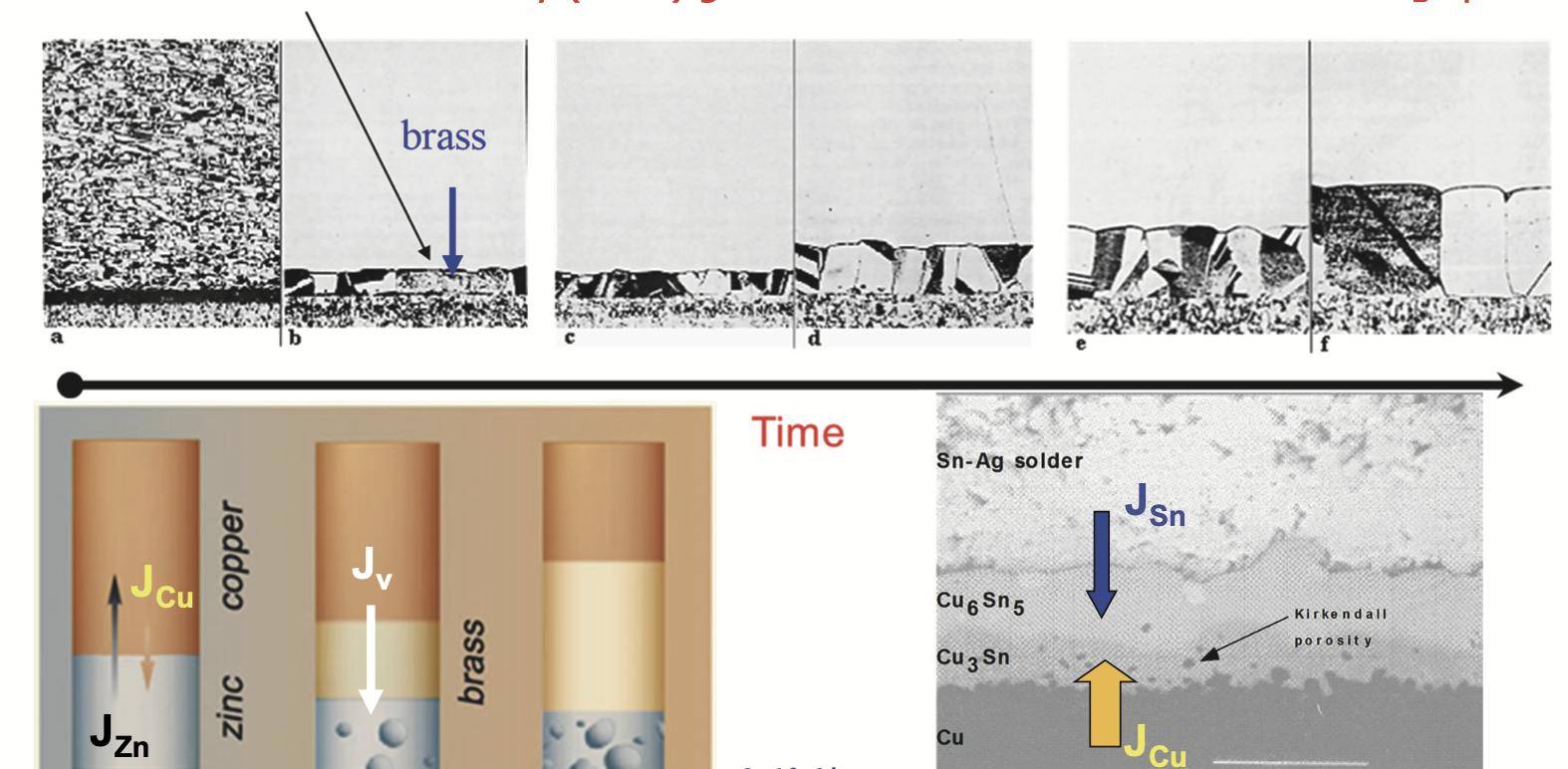
Key observation
- In diffusion couple, markers move relative to lab frame
- Indicates unequal intrinsic fluxes in lattice frame
C-frame vs V-frame fluxes
C-frame (lattice frame)
- net lattice flux can be nonzero: \(J_V^*\neq 0\)
V-frame (lab frame)
\[ J_A^V = -J_B^V,\qquad J_V^V = 0 \]
Interpretation
- \(J_V^*\neq 0\) but \(J_V^V=0\) implies defect accumulation / depletion
Kirkendall effect: physical meaning
Experimentally measured lattice shift
- Markers track lattice (or marker plane)
- Unequal intrinsic fluxes \(\Rightarrow\) vacancy flux
- Vacancy imbalance \(\Rightarrow\) defect accumulation in control volume
- Can produce porosity (Kirkendall voids)
Kirkendall effect: analog

- A diffuse faster than B across the membrane
- \(p_i = c_i RT\)
- Fixed membrane 👉 expanding voids
Kirkendall effect: simulations
See simulation of vacancy mechanism
Credit: Dissemination of IT for the Promotion of Materials Science (DoITPoMS), University of Cambridge
Remaining question 2: interstitial diffusion setup
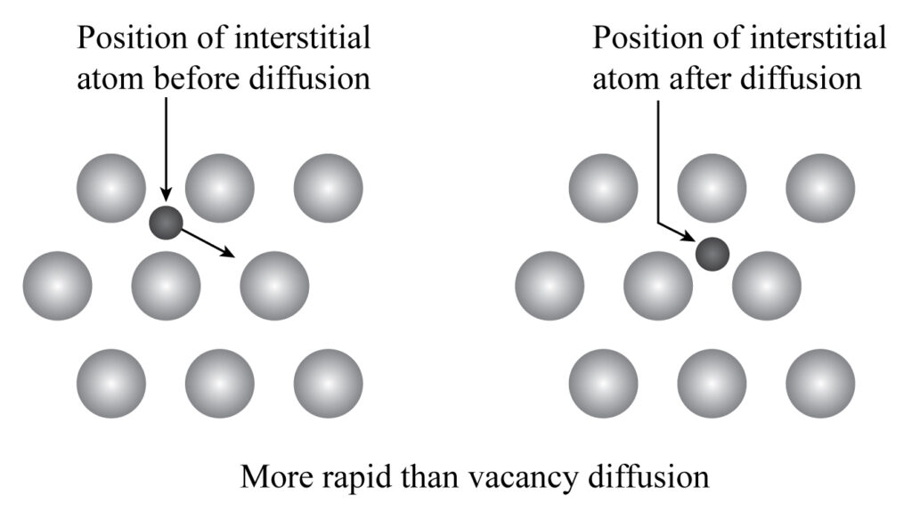
Model ideas:
- species 1 diffuses through sites of 2 (interstitial)
- atoms of 2 are much heavier than 1
- what is the interdiffusivity \(\tilde{D}\)?
Mobility and diffusivity in C-frame
C-frame velocity
\[ v_s^* = \frac{M_1}{c_1}\nabla \mu_1 \]
Then
\[ D_1 = M_1 k_B T \]
and (using Onsager coefficient notation)
\[ D_1 = \frac{L_{11}}{c_1} k_B T \]
Connection
- this matches Nernst–Einstein type relation
V-frame analysis
Special Case: Diffusivity of 2 → 1 with \(D_2=0\)
- species 2 immobile: $D_2=0
- drift velocity related to \(\partial c_1/\partial x\)
- similar to “diffusion through solvent” in mass transfer
V-frame: effective diffusivity
The interdiffusivity now becomes:
\[\begin{align} \tilde{D} &= D_1 \Omega_2 c_2 \\ &= D_1 x_2 \end{align}\]- \(x_2\) is the fraction of lattice particles (usually 1).
- interdiffusivity depends on “how many sites” the smaller species can use
- this expression only applicable for interstitial diffusion!
Driving forces beyond chemical potential
We often used \(\mu_i\) as driving force for diffusion, but other contributions exist.
Generalized “diffusion potential”:
\[ \Phi_i = \mu_i + \sum_j \eta_j \]
- vacancy mechanism / site availability
- electromigration
- external pressure / stress effects
- capillarity / surface curvature effects
- etc.
How do we determine \(D\)?
General experimental workflow:
- impose initial concentration + geometry
- evolve for time \(t>0\)
- measure profile \(c(x,t)\) (or length scale)
- fit to model solution \(\Rightarrow D\)
Forward problem vs inverse problem
Given
- geometry + initial/boundary conditions
- candidate \(D\)
Predict
- concentration profile \(c(x,t)\)
Inverse
- infer \(D\) from measured \(c(x,t)\)
What do we learn in the following lectures?
We want analytical + numerical solutions to the diffusion equations (Fick’s laws)
Start with steady state, then non-steady state.
Covering general formula, and geometries
Fick’s second law (1D, constant \(D\))
Assuming homogeneous isotropic constant \(D\)
\[ \frac{\partial c}{\partial t}=D\frac{\partial^2 c}{\partial x^2} \]
To solve we must specify
- initial condition: \(c(x,0)\)
- boundary conditions: \(c(0,t)\), \(c(L,t)\) or flux BC
Part I: steady state diffusion
Steady state
\[ \frac{\partial c}{\partial t}=0 \quad\Rightarrow\quad \nabla^2 c = 0 \]
This is Laplace equation, having solution in 1D:
\[ \frac{d^2 c}{dx^2}=0 \Rightarrow c(x)=C_1 x + C_2 \]
1D steady state: Dirichlet BC example
If \(c(0)=c^0\) and \(c(L)=c^L\)
Then
\[ c(x)=c^0+\frac{c^L-c^0}{L}x \]
and flux
\[ J=-D\frac{dc}{dx} = -D\frac{c^L-c^0}{L} \]
Cylindrical steady state (radial)
For axisymmetric \(c=c(r)\)
\[ \nabla^2 c=\frac{1}{r}\frac{d}{dr}\left(r\frac{dc}{dr}\right)=0 \]
Integrate twice
\[ c(r)=k_1\ln r+k_2 \]
Cylinder: apply BC at \(r_1, r_2\)
If \(c(r_1)=c_1\) and \(c(r_2)=c_2\)
Then
\[ c(r)=c_1+\frac{c_2-c_1}{\ln(r_2/r_1)}\ln\left(\frac{r}{r_1}\right) \]
Spherical steady state (radial)
For \(c=c(r)\)
\[ \nabla^2 c=\frac{1}{r^2}\frac{d}{dr}\left(r^2\frac{dc}{dr}\right)=0 \]
Integrate to get
\[ c(r)=-\frac{k_1}{r}+k_2 \]
Sphere: apply BC at \(r_1, r_2\)
If \(c(r_1)=c_1\), \(c(r_2)=c_2\)
One convenient form
\[ c(r)=c_1+\frac{c_2-c_1}{\left(\frac{1}{r_2}-\frac{1}{r_1}\right)} \left(\frac{1}{r}-\frac{1}{r_1}\right) \]
Spatially varying diffusivity in steady state
Notes: still solvable if \(D\) depends on 1 variable (e.g. \(x\) or \(r\))
Steady 1D with constant flux \(J\)
\[ J=-D(x)\frac{dc}{dx}=\text{const} \]
So
\[ \frac{dc}{dx}=-\frac{J}{D(x)} \Rightarrow c(x)=c(x_0)-J\int_{x_0}^x\frac{1}{D(\xi)}\,d\xi \]
Often requires numerical integration for \(D(\xi)\).
- Dirchlet boundary 👉 directly integration
- Neumann boundary 👉 need to fix \(dc/dx\) at boundary
Part II: non-steady state diffusion
Different strategies
- superposition with known “source” solutions
- separation of variables (finite domains)
- Laplace transform (initial condition handling)
- numerical methods (general geometry / \(D(c)\))
Method 1: superposition of known solutions
Use linearity of diffusion equation
If \(c_a\) and \(c_b\) satisfy the PDE and BCs, then
\[ c = c_a + c_b \]
also satisfies (with compatible IC/BC decomposition).
Infinite space: half-half situation
Geometry: \(x\ge 0\)
I.C.
- \(c(x<0,t=0)=c_L\)
- \(c(x>0,t=0)=c_R\)
Solution form
\[ c(x,t)=\frac{c_L + c_R}{2} + \frac{c_L-c_R}{2}\,\operatorname{erf}\left(\frac{x}{\sqrt{2Dt}}\right) \]
How do we get here?
Limits and checks
- \(t\to 0^+\): \(\operatorname{erfc}(x/(2\sqrt{Dt}))\to 0\) for \(x>0\) ⇒ \(c\to c_B\)
- \(x\to 0\): \(\operatorname{erfc}(0)=1\) ⇒ \(c(0,t)=c_A\)
- \(x\to\infty\): \(\operatorname{erfc}(\infty)=0\) ⇒ \(c\to c_B\)
Next steps
- Apply these solutions to real diffusion experiments
- Extract \(D\) by fitting measured \(c(x,t)\)
- Extend to variable \(D(c)\) and coupled diffusion (later)
Summary
- The Kirkendall effect reveals differences between lattice and lab reference frames
- Steady-state diffusion problems reduce to Laplace equations with geometry-dependent solutions
- Non-steady diffusion problems can be solved using Gaussian and error-function solutions
- Separation of variables and Laplace transforms provide general tools for solving diffusion equations