MATE 664 Lecture 12
Recitation 1: Kinetics Fundamentals & Diffusion Theory
- Slides 👉 Open presentation🗒️
- PDF version of course note 👉 Open in pdf
- Handwritten notes 👉 Open in pdf
Learning outcomes
This is a recitation class. We will review the main topics covered in the course so far.
After this lecture, you will be able to:
- Recall the major topics covered in the kinetics course
- Describe links between irreversible thermodynamics and kinetics
- Identify analogies between diffusion and other kinetic problems
- Interpret important charts used in diffusion analysis
- Apply course ideas to modern materials research examples
Outlines
- Kinetics \(\approx\) non-equilibrium –> Equilibrium L01
- How to describe non-equilibrium process: Force–flux relation L02 & L03
- Diffusion laws from driving force L04 & L05
- Solving Fick’s equations L06 & L07
- Numerical solution to Fick’s equations L08
- Atomic models for diffusion – Einstein relations L08 & L09
- Diffusion in ideal crystals L10 & defects/short-circuit L11
Conceptual difference: kinetics vs thermodynamics

Entropic view of irreversible thermodynamics
- Any non-equilibrium system going back to equilibrium 👉 entropy generation
- For local system, entropy generation is always non-zero
- Entropy can flow between local systems 👉 root cause of diffusion
\[ \dot{\sigma} = \frac{\partial s}{\partial t} + \nabla\cdot\vec{J}_{s} \geq 0 \]
Entropy flux and generation
- Entropy in the system is nothing but some descriptor of how energy and quantities flow
- Flow of entropy ⇔ Flow of quantities
- Entropy generation ⇔ Magnitude of quantity flow
Quantity – flux – potential relation
- Link in thermodynamics \[ ds = \frac{1}{T}du - \frac{p}{T}dv - \sum_i \frac{\psi_i}{T} d\xi_i \]
- \(\xi_i\): extensive variables
- volume \(v\)
- charge \(q\)
- concentration \(c\)
- surface area \(A\)
- dipole moment \(\mathbf{p}\)
- magnetic moment \(\mathbf{b}\)
- \(\psi_i\): conjugate intensive variables
- pressure \(p\)
- electric potential \(\phi\)
- chemical potential \(\mu\)
- surface energy \(\gamma\)
- external electric field \(\mathbf{E}\)
- magnetic field \(\mathbf{H}\)
Each \((\psi_i,\xi_i)\) pair contributes to entropy change.
Flux – potential relation: driving force
- Extensive quantities: \(\xi_i\)
- Conjugate driving forces: \[ \vec{F}_i \equiv - \nabla \psi_i \]
- Associated fluxes: \(\vec{J}_i\)
Matrix Form
\[ \vec{J} = \mathbf{L}\,\vec{F} \]
equivalent: \[ \vec{J}_i = \sum_j L_{ij}\,\vec{F}_j \]
Kinetics vs thermodynamics: behaviour
- Probability follow Boltzmann distribution \(p \propto \exp\left(-\frac{E + C N}{T}\right)\)
- Scaled potential / entropy \(C = T \mu = T \partial S/\partial N\)
Demo link Copyright: Vilas Winstein (UC Berkeley)
Mass transfer from driving force
Chemical potential \(\mu = \left(\frac{\partial U}{\partial N}\right)_{S,V} = \left(\frac{\partial G}{\partial N}\right)_{P,T}\)
\(\mu\) is driving force for mass transfer / diffusion
Entropy production due to diffusion: \[ T\dot{\sigma} = -\vec{J}_m \cdot \nabla \mu \]
Linear law: \[ \vec{J}_m = -L_{MM}\nabla \mu \]
\(L_{MM}\): phenomenological mobility coefficient
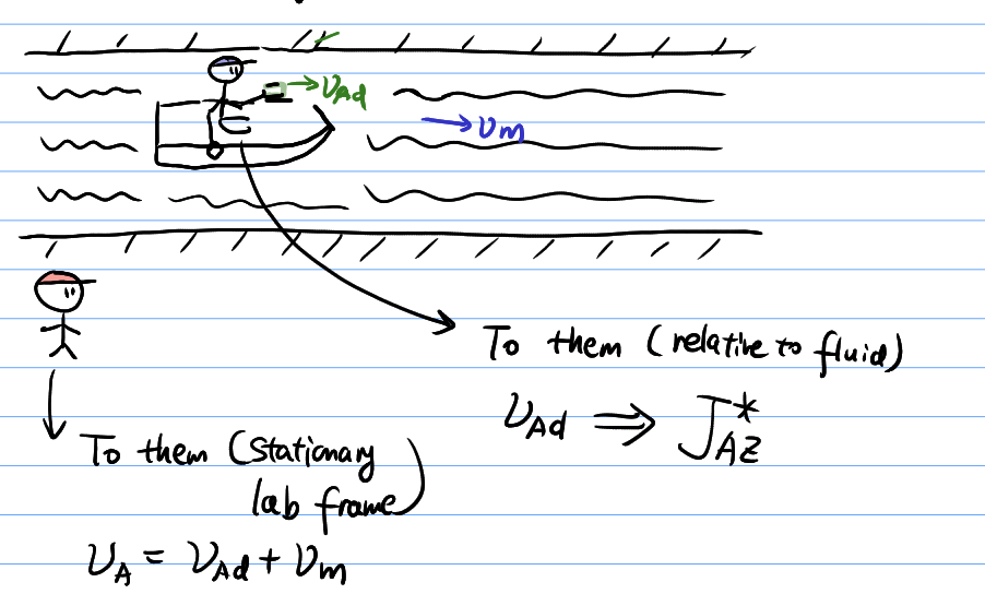
Macroscopic mass transfer: diffusivity – mobility
Force balance and drift velocity (\(M\): mobility): \[ v = M \nabla \mu \]
Mass flux: \[ \vec{J} = c v = -M c \nabla \mu \]
Diffusion coefficient: \[ D = M k_B T \]
Solving mass transfer: Fick’s first law
- Substitute \(\mu\) with \(c\)
- Works for ideal mixture / dilute system
- Isotropic medium (\(D_{\alpha \beta}=D=\text{Const}\))
- Concentration gradient is a special case of \(\nabla \mu\)
For species \(i\) \[ \vec{J} = -D \nabla c \]
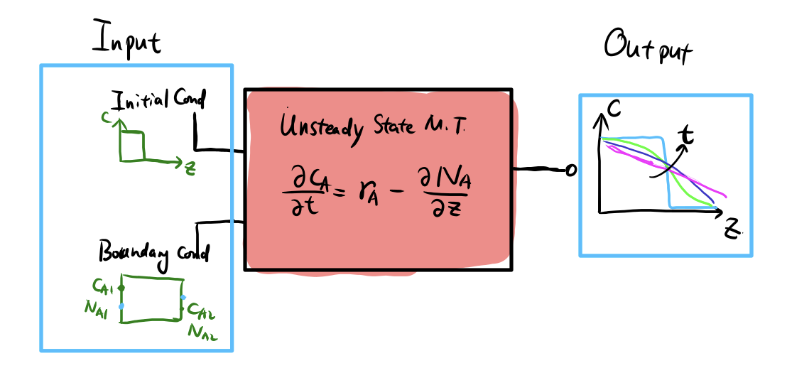
Solving mass transfer: Fick’s second law
Mass conservation (no source term) \[ \frac{\partial c}{\partial t} = -\nabla \cdot \vec{J} \]
Substitution: \[ \frac{\partial c}{\partial t} = \nabla \cdot (D \nabla c) \]
If \(D_i\) is constant: \[ \frac{\partial c}{\partial t} = D_i \nabla^2 c \]
- \(\nabla^2\): Laplace operator
Overview of solutions to mass transfer
Using diffusivity \(D\): different scenarios
| Diffusivity | Frame | Meaning |
|---|---|---|
| \(D_i^{*}\) | lattice | tracer / self-diffusion |
| \(D_i\) | C-frame | intrinsic diffusivity |
| \(\tilde{D}\) | V-frame | interdiffusivity |
Comparison between C- and V-frame
Implications of V-frame interdiffusion
Kirkendall effect
- Movement of interface
- Creation of vacancy voids
Darken’s equation for interdiffusion
Flux form: \[ J_i^{V} = -\tilde{D} \frac{\partial C_i}{\partial x} \]
Interdiffusivity: \[ \tilde{D} = D_1 X_2 + D_2 X_1 \]
Solving Fick’s equation
- Steady-state solution
- Geometry (planar / spherical / cylindrical)?
- Integration over non-isotropic
- Time-dependent (unsteady-state) solution
- Analytical: semi-infinite / point source
- Superimposition of BC and solutions
- Separation of variables method – Fourier transform
- Laplace transform – analysis of temporal decay
Finite difference for Fick’s equation
- Diffusion length scale \(L_D \approx \sqrt{4Dt}\)
| derivative | finite-difference approximation | scheme |
|---|---|---|
| \(\displaystyle \frac{\partial c}{\partial t}\) | \(\displaystyle \frac{c(i,\,j+1) - c(i,\,j)}{\Delta t}\) | forward (time) |
| \(\displaystyle \frac{\partial c}{\partial x}\) | \(\displaystyle \frac{c(i+1,\,j) - c(i-1,\,j)}{2\Delta x}\) | central (space) |
| \(\displaystyle \frac{\partial^2 c}{\partial x^2}\) | \(\displaystyle \frac{c(i+1,\,j) - 2c(i,\,j) + c(i-1,\,j)}{(\Delta x)^2}\) | central (space) |
MOL algorithm (explicit time marching)
- Define spatial grid with \(x_i\) (\(N\) points), choose \(\Delta x\)
- Apply boundary conditions at \(i=0\) and \(i=N\)
- Discretize spatial derivatives using central difference
- Obtain ODE system for \(c(i,t)\)
- Choose time step \(\Delta t\)
- Advance solution in time using forward Euler:
Macroscopic \(D\) ⇔ atomic movements
- Einstein relation: from continuum solution <–> diffusivity
- Random walk model (moluchowski): diffusivity from probability model
- Same conclusion
\[ D = \frac{\Gamma \langle r^2\rangle}{2d} \]
- 3D: \(d=3\)
- 2D: \(d=2\)
- 1D: \(d=1\)
Diffusivity in different environments / states
All follow Einstein relation \(D = \frac{\Gamma \langle r^2\rangle}{6}\)
- Gas: kinetic theory (\(T, P\))
- Liquid: Stokes-Einstein equation (\(\mu, M, R\))
- Solid: activation energy / potential well (\(S^m, H^m\))
Diffusion in solid: general equation
- Vacancy mechanism
Diffusion in ionic crystals
- Extrinsic: vacancy dominated by doped materials
- Low-\(T\) regime (high \(1/T\))
- Intrinsic: vacancy dominated by thermal dissociation
- High-\(T\) regime (low \(1/T\))
Diffusion in imperfections
- Generally \(D^{\text{imp}} \gg D^{XL}\)
- Shortcuts in diffusion pathways
- Lengthscale comparison
Seminal Topics In Diffusion
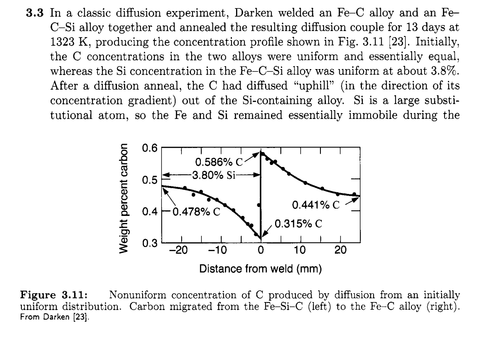
Up-hill diffusion
- Can diffusion happen against concentration gradient?
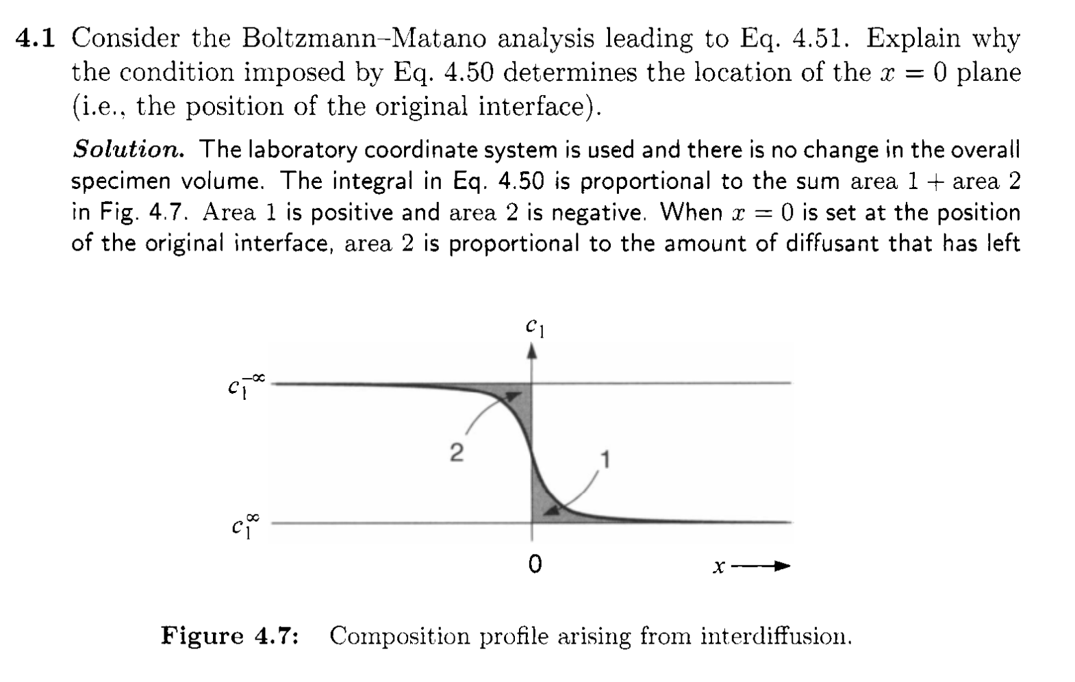
Determination of diffusion in varying \(D\) system
- Boltzmann-Matano analysis of interdiffusion
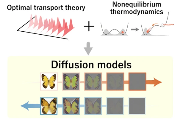
Diffusion models in machine learning
- AI image generation follows a diffusion process!
What to learn next
In the second half of the course, we will cover the following questions
- How do materials evolve when chemical potentials are not at equilibrium?
- In-depth study of phase diagrams
- Continuous phase transformation: spinodal decomposition
- Phase transformation with barrier: nucleation
- How do material interface evolve in non-equilibrium process?
- Heat / mass-transfer at interfaces: solidification
- Surface-energy-mediated transformation: sintering
- Interplay of diffusion & reaction: aggregation phenomena
- How do we simulate / predict material kinetics?
- Macroscopic pattern formation: phase-field method
- Kinetic Monte-Carlo (KMC) simulations
- Molecular dynamics (MD) simulations
- Obtaining thermodynamic parameters from first principles calculations and machine learning
Summary
- This recitation reviewed the major kinetics topics covered in the first half of the course
- Irreversible thermodynamics provides a common framework for diffusion and related kinetic problems
- Diffusion concepts, solution methods, and atomistic pictures connect across many materials systems