MATE 664 Lecture 17
Growth Phenomena: Coarsening
- Slides 👉 Open presentation🗒️
- PDF version of course note 👉 Open in pdf
- Handwritten notes 👉 Open in pdf
Learning outcomes
After this lecture, you will be able to:
- Recall coarsening as a surface-energy-induced growth phenomenon
- Recall the main assumptions of coarsening theory
- Identify the competition between diffusion and reaction-rate control
- Analyze particle size distribution functions during coarsening
Recap: continuous and discontinuous phase transformation
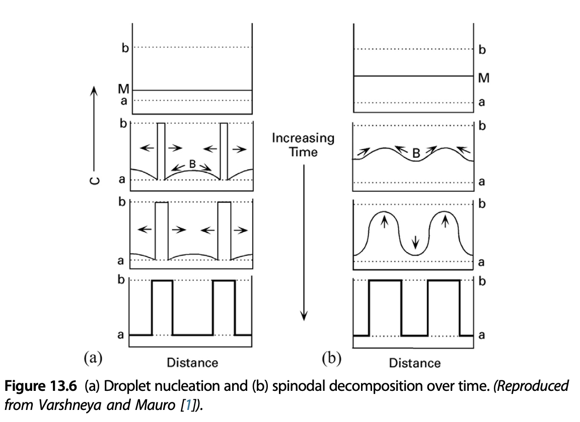
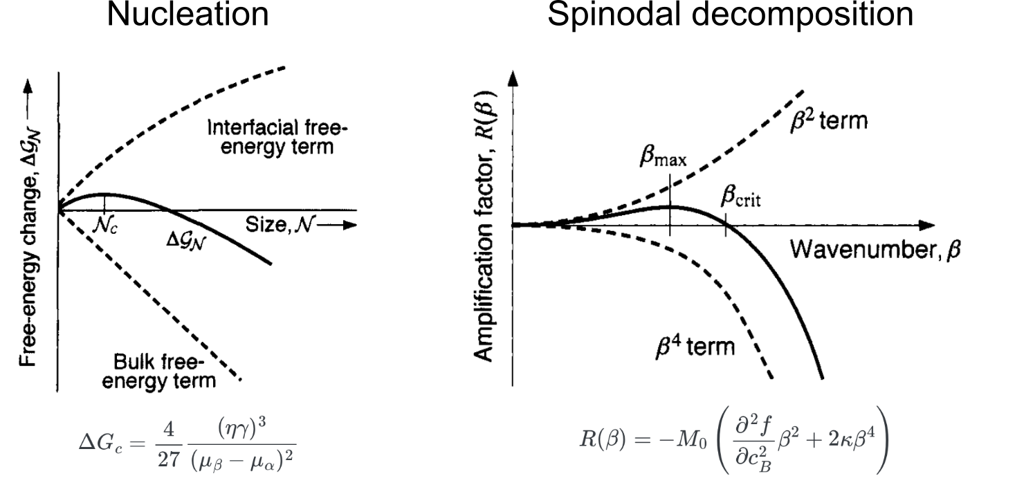
Recap: growth barrier comparison
Recap: growth stages in a nucleation process
- What happens to stages III and IV? 👉 Coarsening process

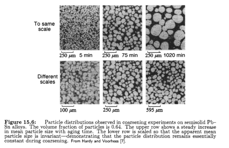
Coarsening: growth mechanism involving particle size distribution
Pb-Sn alloy coarsening experiment shows that particle distribution remains almost constant (Stage III)
Another angle: Ostwald ripening
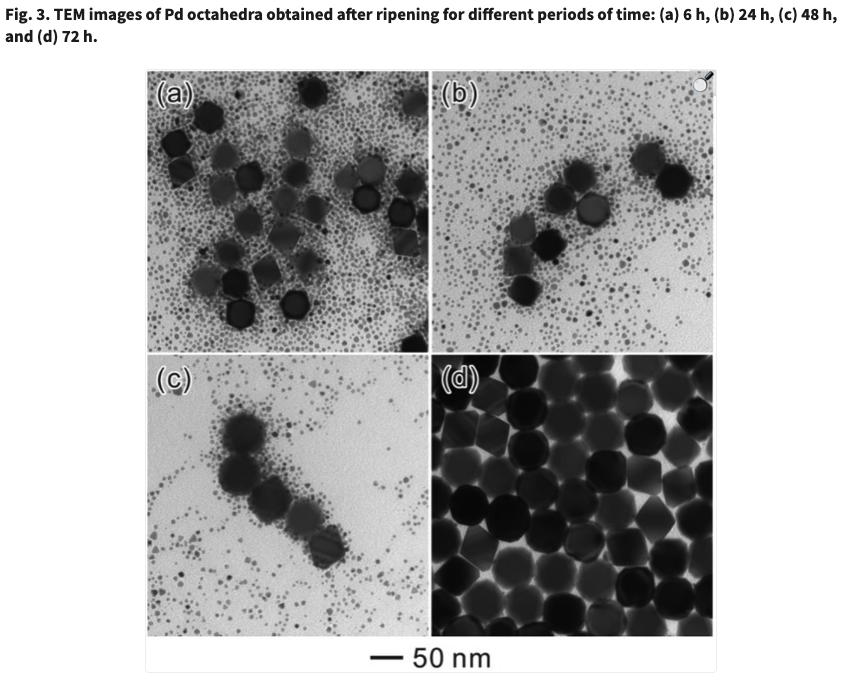
Experimental observation of small Pt particles are “absorbed” by the larger particles (Stage IV)
Analog: two-balloon experiment
- The effect of curvature on the total free energy is analogous to the two-balloon experiment
- The driving force is capillarity
- YT Video
Capillarity as a driving force
The term “capillarity” refers to a broad variety of phenomena involving the interface
- Excess free energy caused by surface energy + curvature
- Driving force: minimizing interfacial area
- Morphology change: interfaces will move during the optimization process
- Coarsening: large particles “absorb” small particles; particles do not touch
- Coalescence/sintering: interface between close-contact particles disappear; particles touch and merge
Crash course: interfacial coordinate system
For the interface between A and B that has no parallel movement, the curvature \(H\) depends on the direction of the normal vector \(\mathbf{n}\), so that
\[ p_{\mathrm{A}} - p_{\mathrm{B}} + 2 H \gamma = 0 \]

in either definition, \(p_A > p_B\) (makes sense?)
Crash course: interfacial curvature
The surface curvature \(H\) can be expressed using the two principle radii \(R_{1}\) and \(R_{2}\) of the surface:
\[\begin{align} |H| &= \frac{1}{2}(\frac{1}{R_{1}} + \frac{1}{R_{2}}) \\ &= \frac{1}{2}(\kappa_1 + \kappa_2) \end{align} \]
Capillary force: water droplet situation
Nanoscale droplet will have excessive pressure!

Capillarity as driving force: high level description
The driving force from capillarity \(\Delta f\) is generally the energy change caused by the volume swept out by the interface, so that
\[\begin{align} \Delta f &= \frac{\Delta E}{\text{volume due to moving interface}} \\ \gamma (\kappa_1 + \kappa_2) \end{align} \]The driving force has 2 factors:
- non-zero surface energy \(\gamma\):
- curvatures \(\kappa_1\), \(\kappa_2\) (\(\propto 1/R\))
Coarsening (Ostwald ripening)
The evolution of an inhomogeneous structure in a solid solution or a colloidal system (stages III and IV)
- Feature: small particulates dissolve, and redeposit onto large particulates.
- Driving force: minimization of total interfacial energy.
- Mass transport: driven by curvature-dependent surface potential.
- Size and number of particles change with time.
Classical mean-field theory of coarsening
- Most prominent theory LSW theory (Lifshitz-Slyozov-Wagner, 1961)
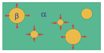
- Spherical \(\beta\) particles embedded in \(\alpha\) matrix in A-B mixture
Key take-aways:
- Eq. concentration at interface: increase on smaller particles
- B atoms: small particle –> matrix –> large particle
- Smaller particles shrink; larger particles grow
Influence of curvature on free energy: Gibbs-Thompson effect
From our balloon analog, curvature-induced pressure for an isotropic sphere is:
\[ \Delta p = p_A - p_B = \gamma(\kappa_1 + \kappa_2) = 2 \frac{\gamma}{R} \]
By adding an B particle in to the \(\beta\) phase, the change of volume is \(\Omega_B\) and there is an increase of free energy \(2 \frac{\gamma \Omega_B}{R}\). The interfacial concentration \(c_B^{\text{eq}}(R)\) is then higher than \(c_B^{\text{eq}}(\infty)\)
\[\begin{align} c_B^{\text{eq}}(R) &= c_B^{\text{eq}}(\infty) \exp(\frac{2 \gamma\Omega_B}{k_B T R}) \\ &\approx c_B^{\text{eq}}(\infty) \left[ \exp(\frac{2 \gamma\Omega_B}{k_B T R})\right] \end{align} \]This is known as the Gibbs-Thompson effect
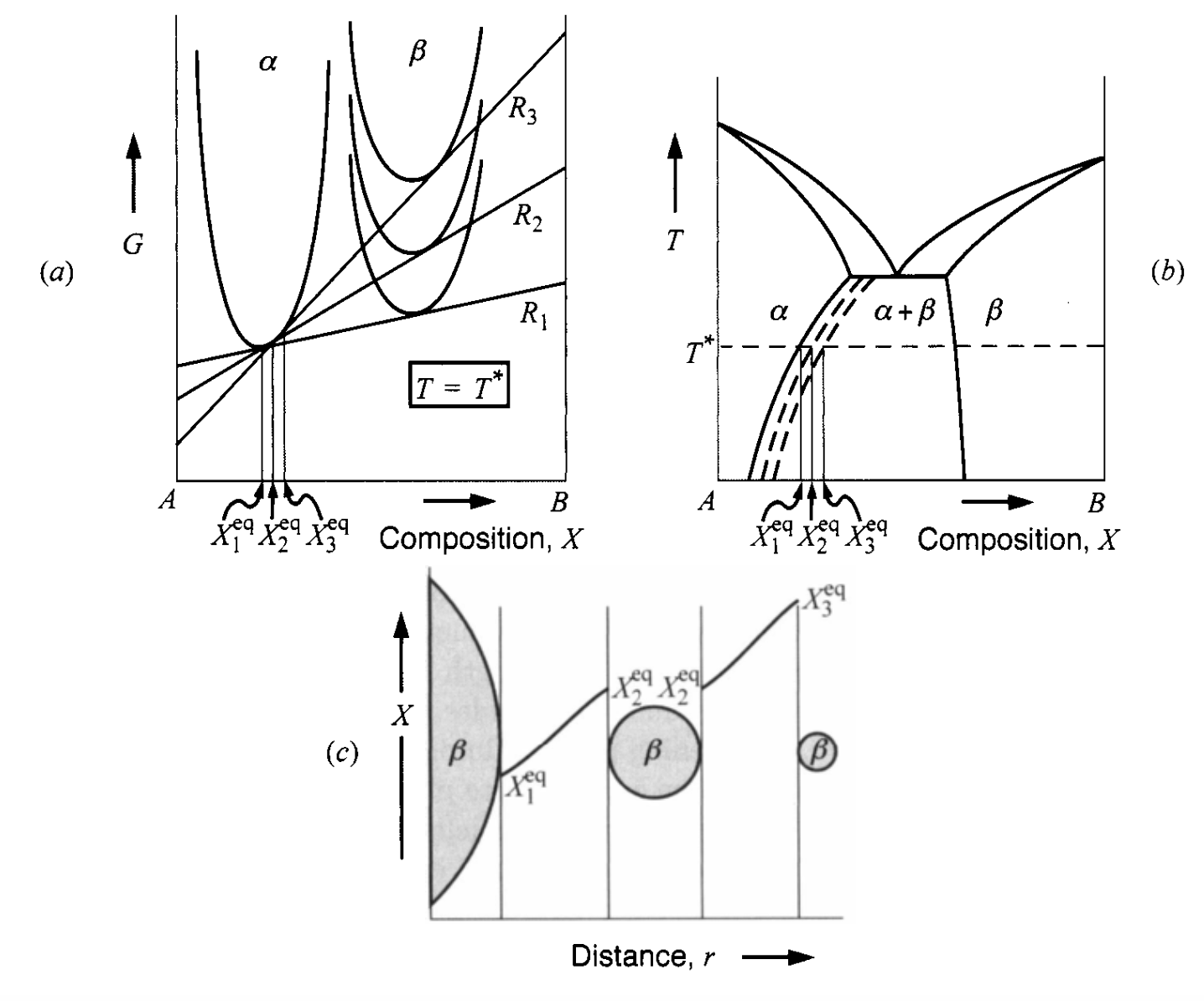
Gibbs-Thompson effect in a phase diagram
- Gibbs-Thompson effect will shift \(\mu_B\) to higher values when particles are smaller
- Difference between interfacial concentration creates a diffusion field!
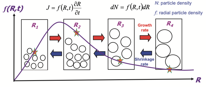
LSW theory: the particle distribution picture
Similar to the nucleation theory where \(J_n\) measures the flux of particle size distribution function \(N(n, t)\), we’re also interested in the particle size distribution over time, \(f(R, t)\), with following components
- distribution (density) function of particle size \(R\): \(f(R, t)\)
- radial particle density between \(R \to R+dR\): \(dN(R\to R+dR, t) = f(R, t)dR\)
- conservation of volume: \(\sum_i R_i^2 \dfrac{dR_i}{dt} = 0\)
The radial distribution function
Compare with the quasi-steady state picture of nucleation in Lecture 14. The R has no cutoff compared with the QSS treatment in constrained growth.
Diffusion-controlled coarsening kinetics
In the diffusion-controlled regime of coarsening, the rate of growth for particles is associated with the surface flux from excess concentration to the bulk.
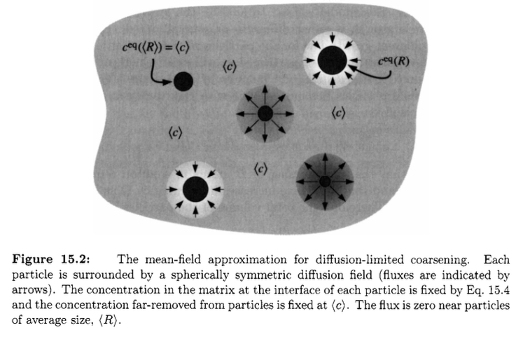
Rate equations in diffusion-controlled regime
- Growth rate from flux onto a sphere
\[ \frac{dR}{dt} = - \tilde{D} \frac{(c^{\text{eq}}(R) - <c>)}{R}\omega_B \]
- Excess surface concentration:
\[ c_B^{\text{eq}}(R) \approx c_B^{\text{eq}}(\infty) \left[ \exp(\frac{2 \gamma\Omega}{k_B T R})\right] \]
- Conservation
\[ \sum_i R(c^{\text{eq}}(R) - <c>) = 0 \]
Diffusion-controlled regime: final results
The growth rate at each \(R\) is:
\[\begin{align} \frac{d R}{d t} &= \frac{2 \tilde{D} \gamma \Omega_B^2 c^{\text{eq}}(\infty)}{k_B T R} \left(\frac{1}{<R>} - \frac{1}{R}\right) \end{align}\]- \(<R>\): average radius of particles. \(f(<R>) = 0\)
- \(R < <R>\): \(dR/dt<0\) 👉 shrink!
- \(R_{\text{max}} = 2 <R>\)
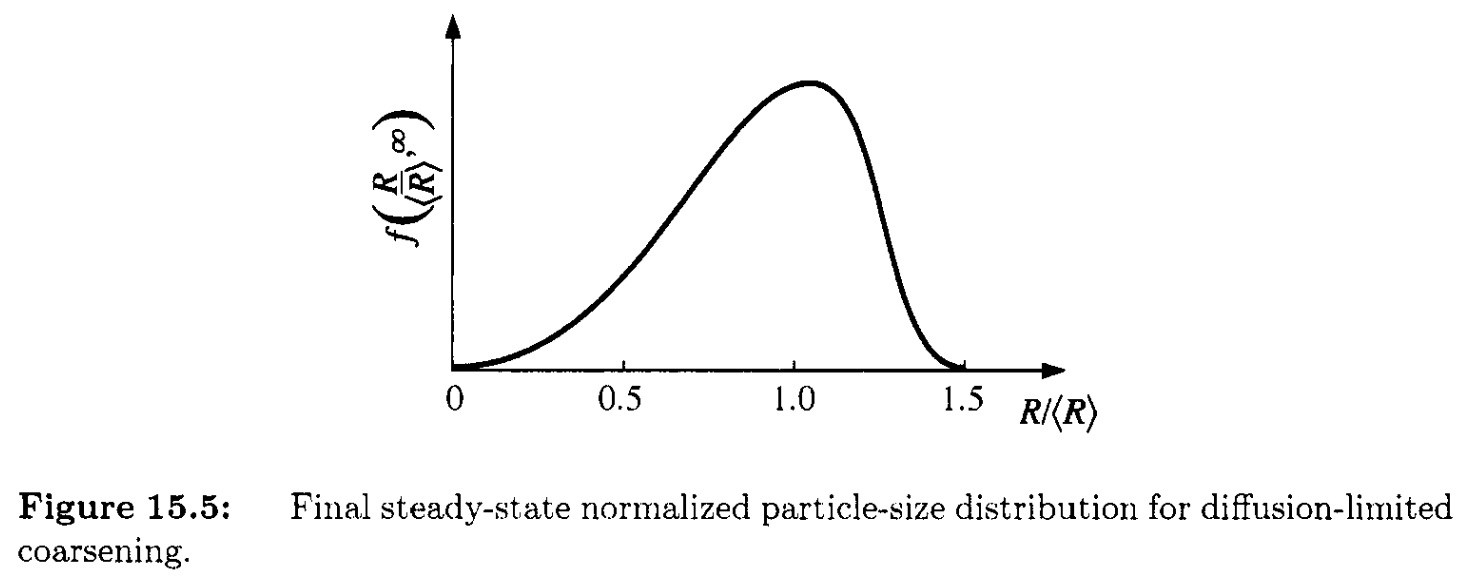
The steady-state particle size distribution
The radius distribution has a very nice feature that even if \(<R>\) grows over time, at steady state, the normalized radius \(R/<R>\) has the same distribution:
- most frequent size \(R \approx 1.13 <R>\)
- no particle larger than \(1.5<R>\) (cutoff)
Diffusion-controlled regime rate law
Power-of-3 law: particle size growth rate
\[\begin{align} <R(t)>^3 - <R(0)>^3 = \frac{8 \tilde{D} \gamma \Omega^2 c^{\text{eq}}(\infty)}{9 kB T} = K_D t \end{align}\]In experiment the measured growth follows \(\langle R \rangle \propto t^{1/3}\). See previous example of Pb-Sn alloy
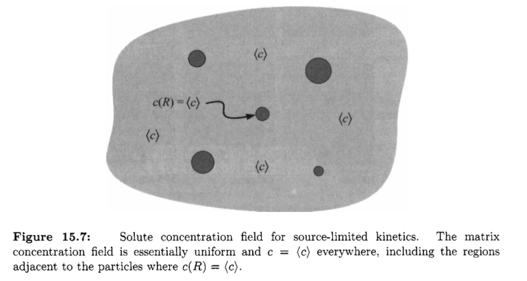
Source-limited growth regime
Another regime is the source-limited coarsening. Diffusion in matrix is very fast and rate limiting step is the source / sink at interface.
Source-limited growth: change of formula
Again, we have curvature-dependent interfacial concentration difference, but the growth rate is purely controlled by the concentration difference!
\[ \frac{d R}{d t} = \frac{2 K c^{\text{eq}}(\infty) \Omega^2 \gamma}{k_B T} (\frac{<R>}{<R^2>} - \frac{1}{R}) \]
- Particle will shrink if \(R < <R^2>/<R>\)
Source-limited growth: change of power law
For source-limited growth, we will have the radius grow in a power-of-2 fashion
\[\begin{align} \langle R^{2}(t) \rangle - \langle R^{2}(0) \rangle &= \frac{64 K c^{\text{eq}}(\infty) \Omega^2}{81 k_B T} \\ &= K_s t \end{align}\]In experiments you will measure that \(\sqrt{\langle R^{2}(t) \rangle} \propto t^{1/2}\), a different power law than the diffusion-controlled growth!
Summary
- Driving force for coarsening: capillarity (surface energy + curvature)
- Key take away from coarsening: particle growth kinetics & size distribution
- Diffusion and rate-limit regimes