MATE 664 Lecture 13
Phase Diagram and Phase Transformation
- Slides 👉 Open presentation🗒️
- PDF version of course note 👉 Open in pdf
- Handwritten notes 👉 Open in pdf
Kinetics of Materials Part II
What topics have we learned so far?
- How to describe kinetic process: irreversible thermodynamics
- What causes nonequilibrium mass transfer: chemical potential as driving force
- Diffusion in materials: Fick’s equations
- Determine diffusivity \(D\): Macroscopic and Microscopic models
What do we study in Part II?
Insights from assignments 1 and 2

Topic 1: phase transformation
Key question: how do materials evolve when chemical potentials are not at equilibrium?
- In-depth study of phase diagrams
- Continuous phase transformation: spinodal decomposition
- Phase transformation with barrier: nucleation
Topic 2: interfacial phenomena
Key question: how do material interfaces change in non-equilibrium process?
- Solidification: heat / mass-transfer at interfaces:
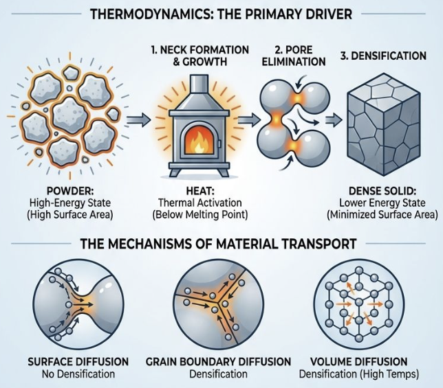
- Sintering: surface-energy-mediated transformation:
Topic 3: analysis of kinetic process in materials
Key question: how do the competition between different effects change the material behaviour?
- Aggregation phenomena: diffusion & reaction of soft materials
- Dendrite formation: morphological control in battery electrodes
- Carrier transport: designing optical materials
Topic 4: simulating kinetic problems
Key question: what methods can we use to simulate kinetic systems, and how good are they?
- Macroscopic transport: phase-field method
- Kinetic Monte-Carlo (KMC)
- Molecular dynamics (MD)
- Thermodynamic parameters from first principles and machine learning
Introduction to phase transformation
Learning outcomes
After this lecture, you will be able to:
- Recall key components of a phase diagram
- Distinguish the meaning of axes in a phase diagram
- Identify key thermodynamic relations from a phase diagram
- Analyze phase transformation regions in a phase diagram
This lecture is adapted from Porter et al. Phase Transformations in Metals and Alloys
What is phase transformation?
Before introducing any fancy terminologies, let’s define a few concepts:
- Phase:
- a region with uniform structure and properties
- Transformation
- a kinetic process to reduce total free energy by turning phases α –> β
- Interface
- a boundary separating two phases
![]()
What can be considered as a phase?
- Mathematically (Landau & Lifshitz 1963), different phases are distinguished by order parameter \(\xi\)
- The molar free energy \(F(T, \xi)\) can be written as a series expansion of \(\xi\)
- \(F\) can be Helmholtz or Gibbs free energy
- 1st order phase transition
- \(F\) is continuous at phase interfaces,
- \(\xi\) has abrupt jump
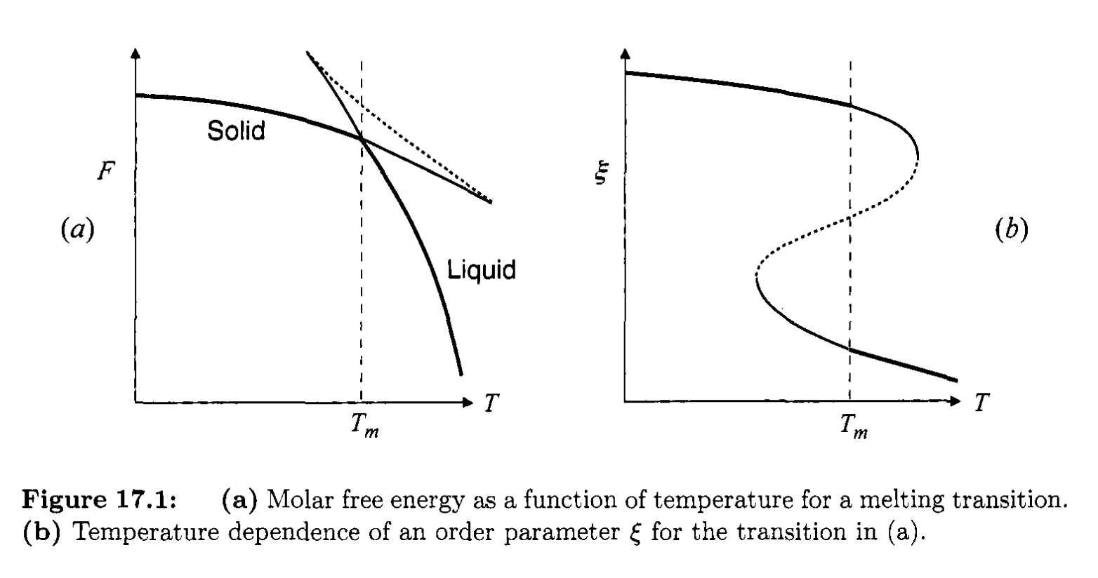
General picture of phase transformation (1st-order)
- Example of solid-liquid transformation (KOM book)
- Order parameter \(\xi\) can be arbitrary
- \(\xi\) always lower on the high-T phase
What quantity can be an order parameter?
Examples of order parameters \(\xi\) (what changes across a phase boundary)
- structure: e.g., fcc \(\leftrightarrow\) bcc
- molar volume \(V_m\): liquid \(\leftrightarrow\) solid
- magnetization \(M\): paramagnetic \(\leftrightarrow\) ferromagnetic
- superconducting order parameter \(\psi\): normal \(\leftrightarrow\) superconducting
Magnetization as order parameter (second-order transition) 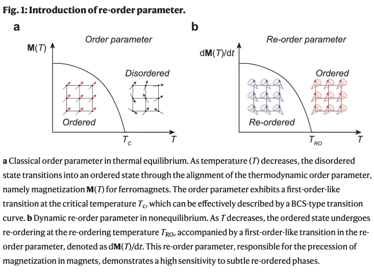
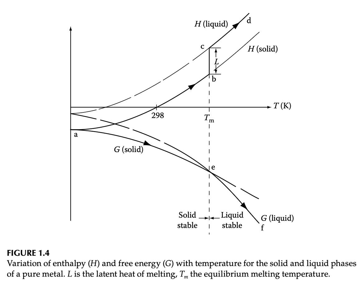
Dissecting the solid-liquid free energy diagram
- Typical \(H\) and \(G\) diagrams for the single-component system
- \(G\) is continuous while \(H\) is discontinuous
- Difference in liquid-solid enthalpy: latent heat \(L\)
How do we get here?
- Enthalpy from specific heat \(C_p\): \(C_p = \left(\dfrac{\partial H}{\partial T}\right)\vert_{p}\)
- Entropy from specific heat: \(\dfrac{C_p}{T} = \left(\dfrac{\partial S}{\partial T}\right)\vert_{p}\)
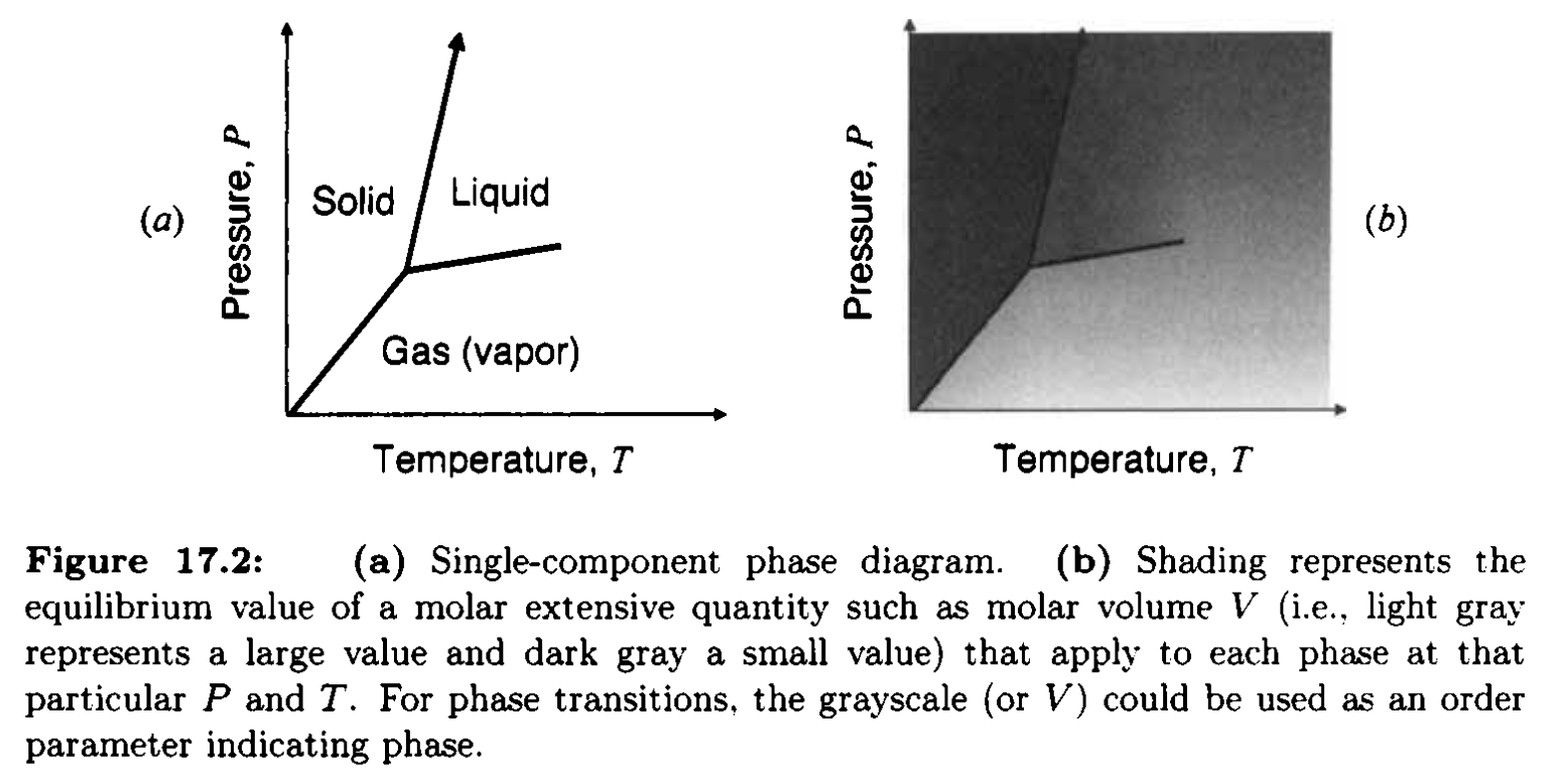
Single-component system: including pressure
- Left to right: increasing \(T\) (melting / evaporation)
- Lower to upper: increasing \(p\) (condensation)
- How do free energy profile look like?
Single-component system: slope of phase boundary
- Phase boundary equilibrium \(G^{\alpha} = G^{\beta}\)
- Slope of \(p-T\) diagram: Clausius-Clapeyron equation
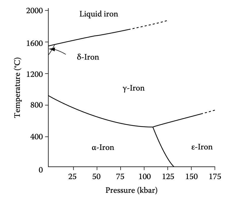
Reading single-component phase diagram (Fe)
- What can we say about the lattice structure about Fe allotropes?
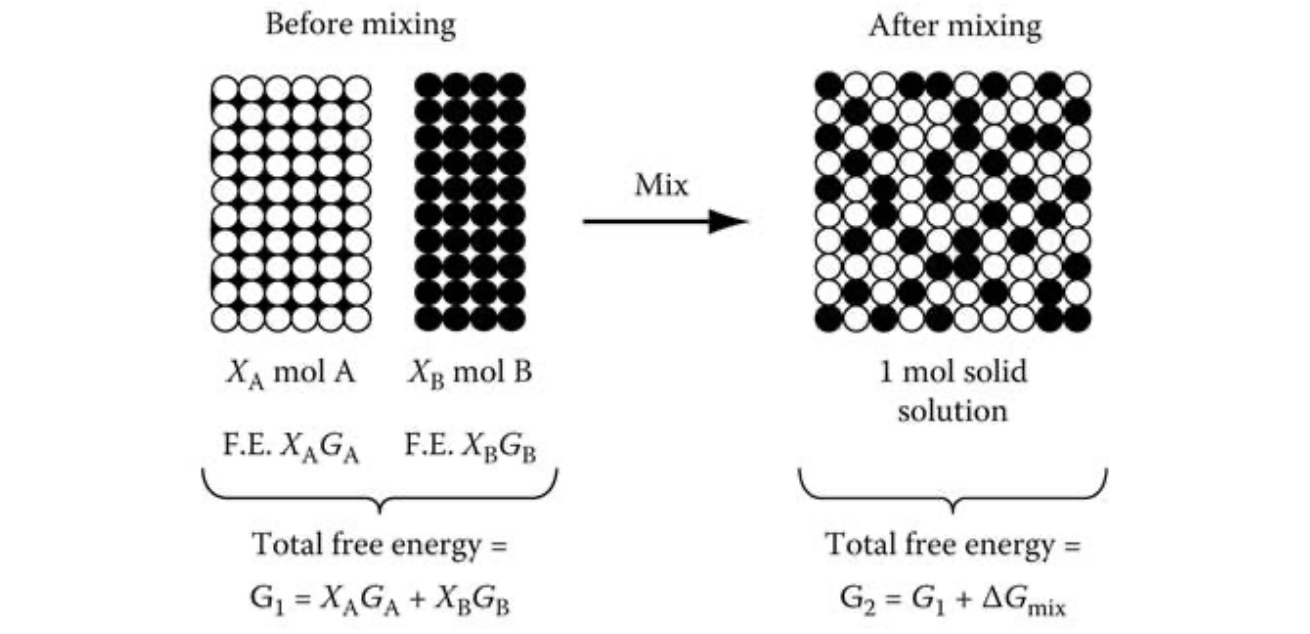
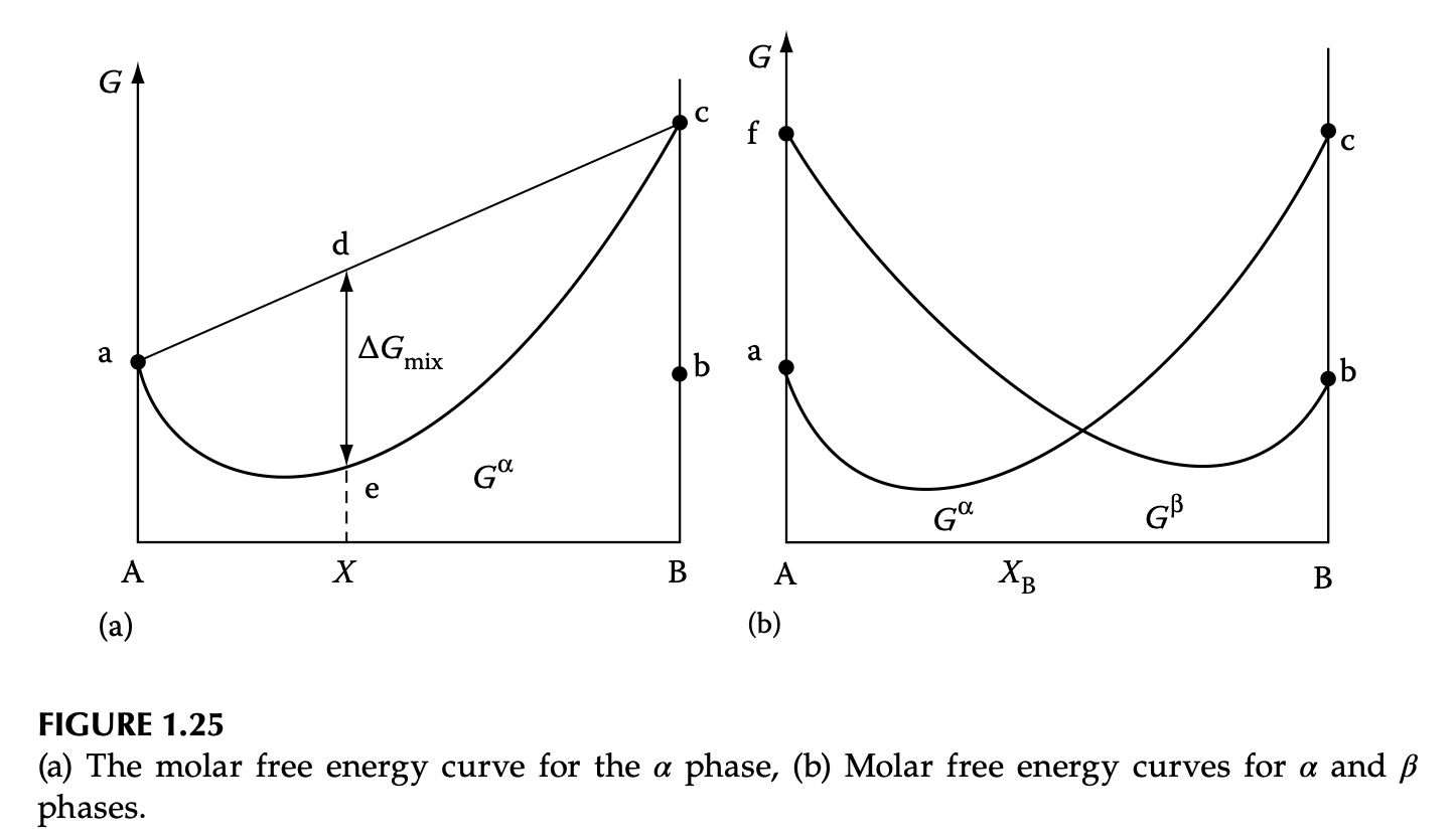
Free energy diagrams of binary mixture
- Mixing of two materials A and B causes free energy to change
- Before mixing, molar free energies \(G_A\), \(G_B\)
- After mixing, molar free energy becomes
Ideal solution: mixing entropy
- In ideal solution \(\Delta G_{\text{mix}} = -T \Delta S_{\text{mix}}\)
- Ideal mixing entropy
\[ \Delta S_{\text{mix}} = -R (X_A \ln X_A + X_B \ln X_B) \]
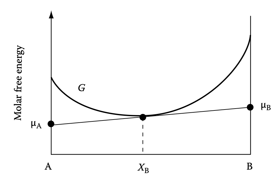
Chemical potential on molar free energy diagram
- Chemical potential from \(G\): \(\mu_A = \left(\frac{\partial G}{\partial X_A}\right)\vert_{T, p, X_B}\)
- Ideal solution: \(\mu_A = G_A + RT \ln X_A\)
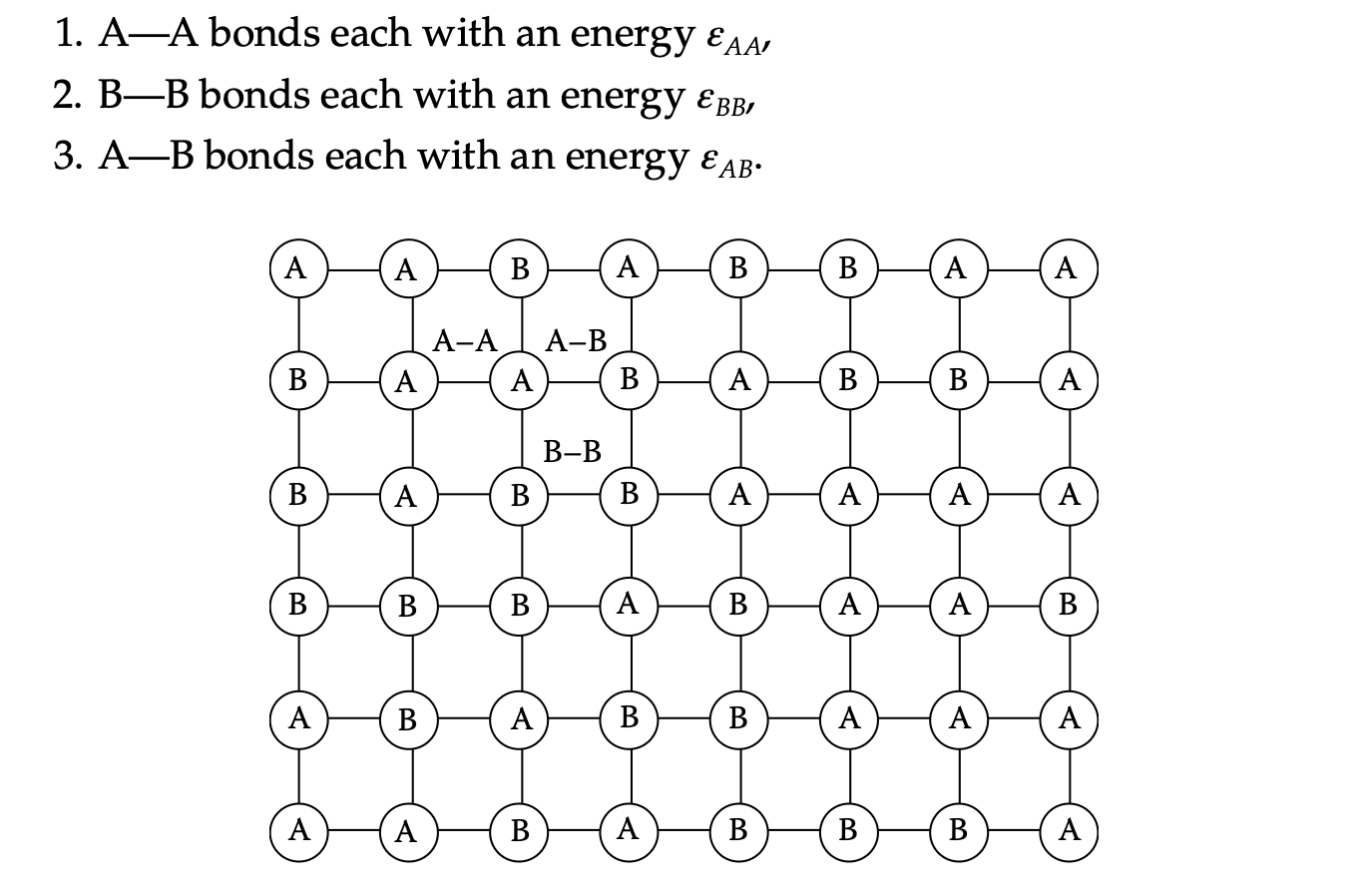
Regular solution: mixing enthalpy
- Generally \(\Delta H_{\text{mix}} \neq 0\)
- Can be expressed by “likeliness” between A-B
\[ \Delta H_{\text{mix}} = N_A z (\varepsilon_{AB} - \frac{1}{2} (\varepsilon_{AA} + \varepsilon_{BB})) X_A X_B \]
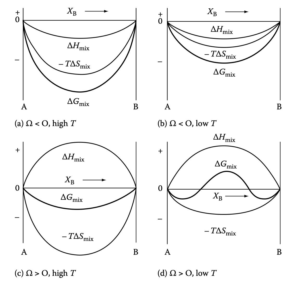
Enthalpic and entropic contributions to mixing
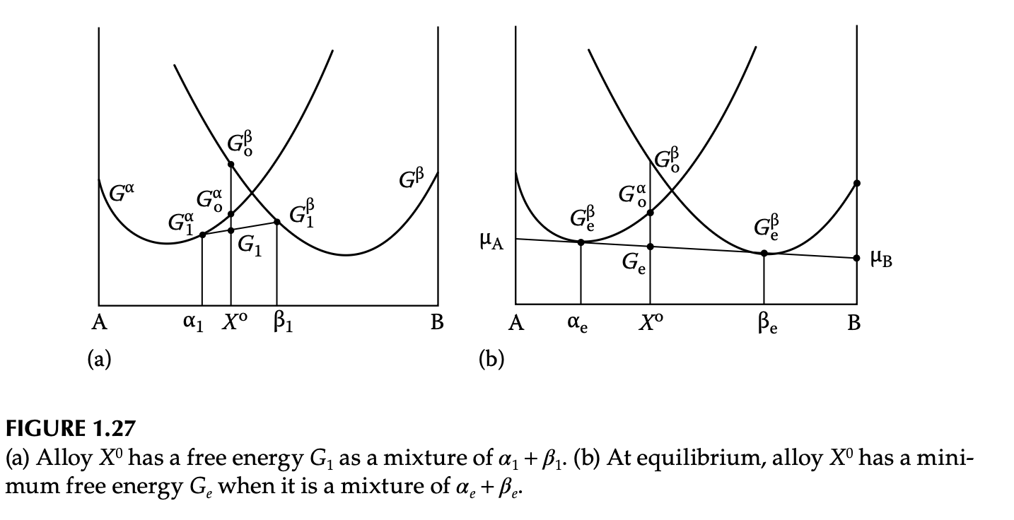
Heterogeneous phase diagram
- At each \(T\), molar free energy of 2 phases are calculated separately
- Imaginary “unstable lattice” for incompatible crystals
- What is the most stable phase at each \(X\)?
Heterogeneous system: equilibrium
- Equilibrium condition (common tangent): \(\mu_A^\alpha = \mu_A^\beta\) & \(\mu_B^\alpha = \mu_B^\beta\)
- Lever rule: graphical explanation
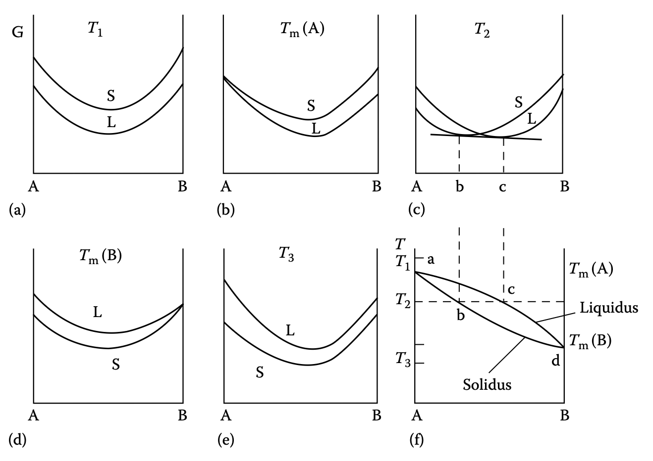
Phase diagram example 1: completely miscible solid & liquid
- E.g. Cu–Ni alloy (fcc)
Phase diagram example 2: miscibility gap
- Solid state \(\Delta H_{\text{mix}} > 0\)
- Will be our example for spinodal decomposition
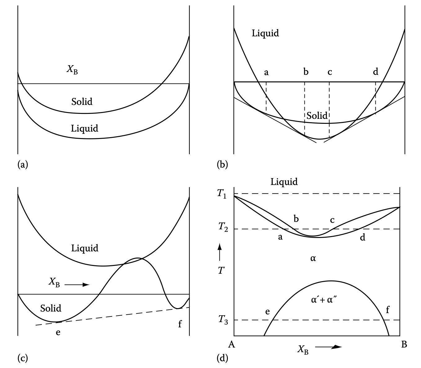
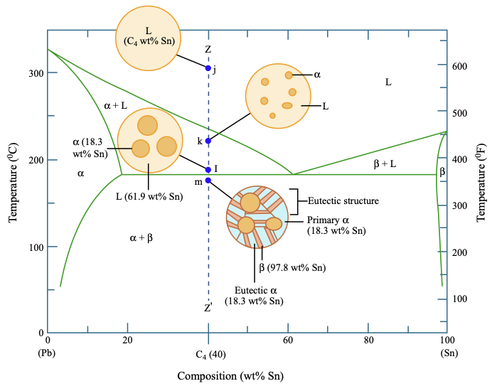
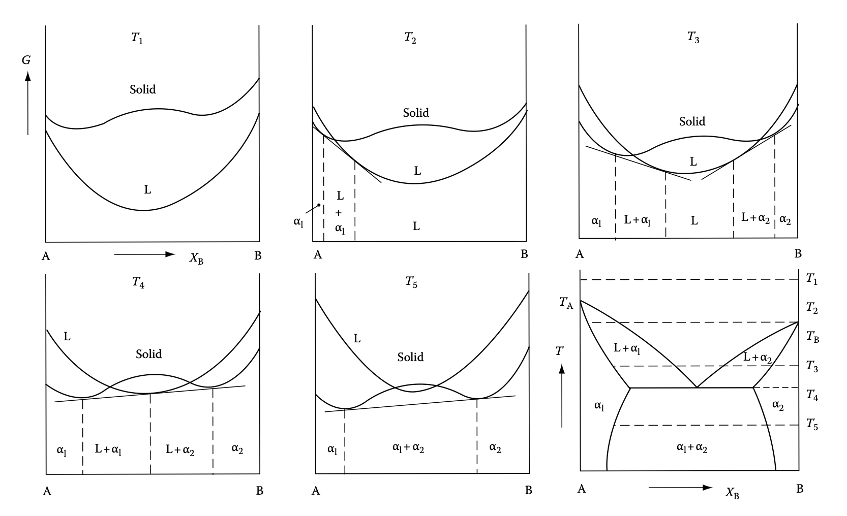
Phase diagram example 3: eutectic alloy (same lattice)
- Eutetic formation due to dominant solid-phase
Additional effects for phase stability
- Phase diagram does not tell everything!
- Stability of a phase depends on
- Molar free energy (what phase diagram tell)
- Interfacial energy (extra work to stablize interface)
- Kinetic stability (metastable & unstable regions)
- Actual important issue for kinetic course
- Interface influence: nucleation theory
- Kinetic stability: spinodal decomposition
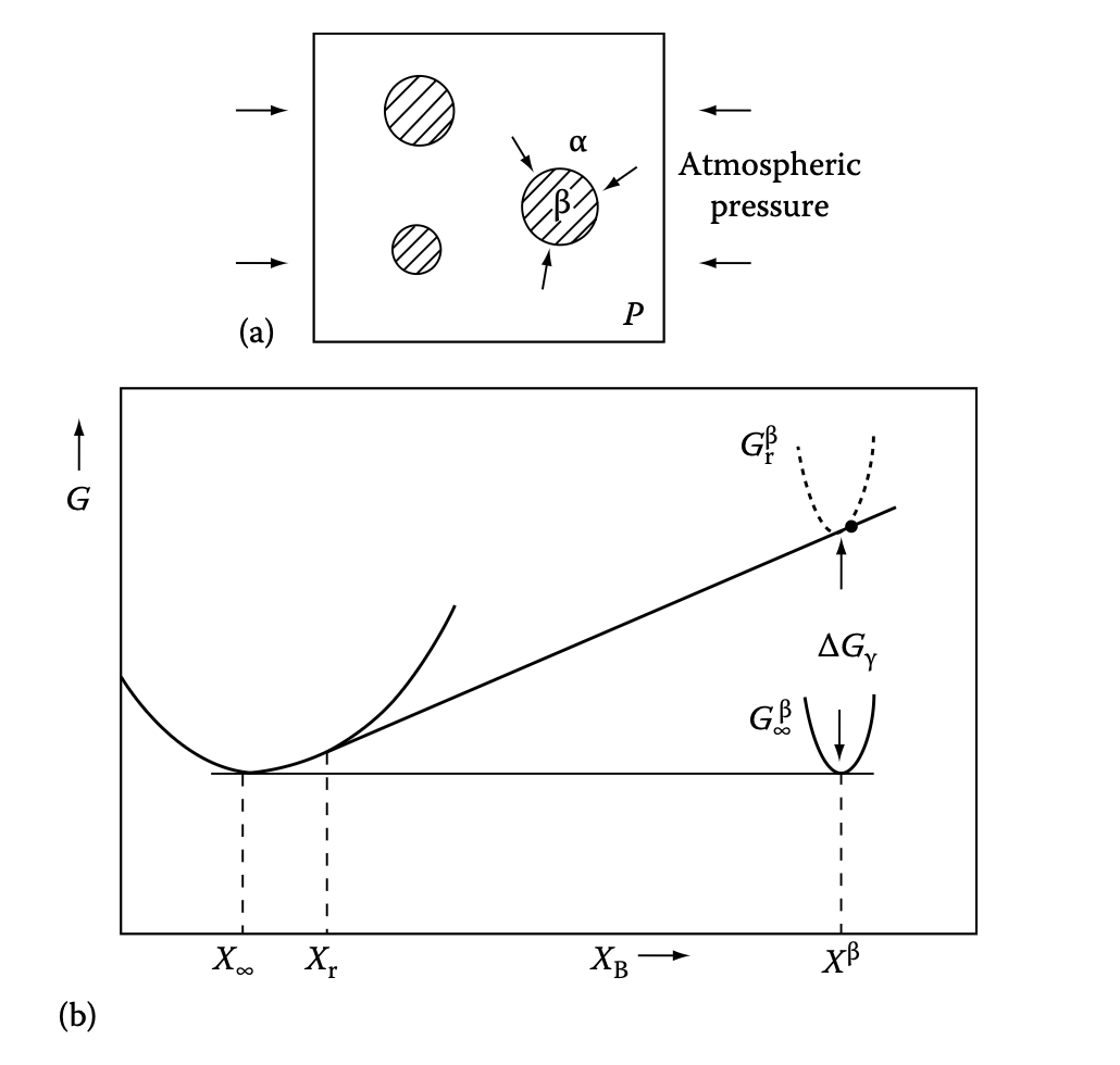
Preview: influence of interfacial energy
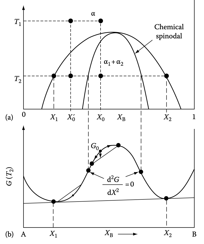
Preview: second-order stability in spinodal decomposition
Summary
In today’s lecture, we overviewed the origin of phase transformation and phase diagram.
- Phase transformation can be described by free energy as function of an ordered parameter
- Equilibrium phase diagram is constructed by the lowest free energy phase
- Free energy of mixing –> chemical potential –> constructing phase diagram
- Basic literacy in phase diagram reading!