MATE 664 Lecture 16
Continuous Phase Transformation: Spinodal Decomposition
- Slides 👉 Open presentation🗒️
- PDF version of course note 👉 Open in pdf
- Handwritten notes 👉 Open in pdf
Learning outcomes
After this lecture, you will be able to:
- Recall the difference between continuous and discontinuous phase transformations
- Describe spinodal decomposition as a continuous phase transformation process
- Identify the chemical-potential driving force in spinodal decomposition
- Analyze the Cahn-Hilliard equation and its gradient driving force
Recall: general picture of phase transformation
Stability regions in \(T-X_{B}\) and \(G-X_{B}\) plots - spinodal: “spine-like” shape in the free energy diagram
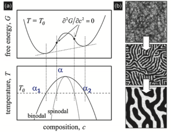
Stability of phase transformation: second derivative of free energy
Taylor expansion of the Gibbs free energy
\[\begin{align} G\!\left(x_B^{0}+\delta x_B\right) &= G\!\left(x_B^{0}\right) + \left.\frac{\partial G}{\partial x_B}\right|_{x_B^{0}}\,\delta x_B + \frac{1}{2}\left.\frac{\partial^{2}G}{\partial x_B^{2}}\right|_{x_B^{0}}(\delta x_B)^2 \nonumber\\ &= G\!\left(x_B^{0}\right) + \frac{1}{2}\left.\frac{\partial^{2}G}{\partial x_B^{2}}\right|_{x_B^{0}}(\delta x_B)^2 \end{align}\]Key questions to be answered for continuous transformation
- Where: which region in a phase diagram does continuous phase transformation occur?
- How: how does the continuous transformation differ from discontinuous one (e.g. nucleation)?
- Why: why do we see the continuous behaviour?
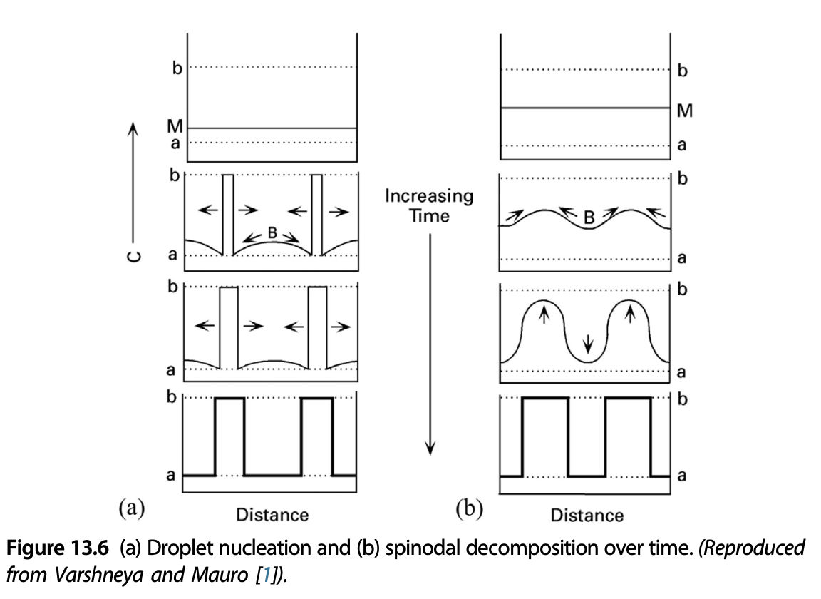
Comparison: nucleation vs spinodal decomposition
Continuous transformation: irreversible thermodynamics view (1)
From Lecture 08 we know the fluxes between an A-B binary mixture follows:
C-frame: \(J_A^C\) & \(J_B^C\)
V-frame: \(J_A^V\) & \(J_B^V\)
Conservation equations
Continuous transformation: irreversible thermodynamics view (2)
Expanding the flux conservation and Gibbs-Duhem equation we get the \(J_B^V\) as
\[\begin{align} J_B^V &= -\Omega^2 (c_A^2 L_B + c_B^2 L_A)(\nabla \mu_B - \nabla \mu_A) \\ &= -\Omega^2 (c_A^2 L_B + c_B^2 L_A)\nabla(\mu_B - \mu_A) \\ &= - M \nabla(\mu_B - \mu_A) \end{align}\]So far this is just a formal diffusion equation using chemical potential driving force
Meaning of \(J_B^V\) equation
- Mobility \(M>0\) satisfies the \(\dot{\sigma}\geq 0\) postulate
- What is \(\mu_B - \mu_A\)? 👉 Slope \(\partial G/\partial X_B\) on the free energy diagram!
- What is \(\nabla(\mu_B - \mu_A)\)? Spatial variation of the \(\partial G/\partial X_B\) driving force
Negative interdiffusivity?
From previous analysis we see that the apparent interdiffusivity \(\tilde{D}\) follows:
\[ \tilde{D} = \frac{M\Omega}{N_0} \frac{\partial^2 G}{\partial X_B^2} \]
- \(\tilde{D} < 0\) 👉 uphill diffusion
- In continuous transformation, we see the local concentration difference amplifies!
- In contrast, normal diffusion \(\tilde{D} > 0\) tries to smoothen the concentration curvature.
Diffusion (homogenization) vs phase separation
Very rough estimation of the composition change using Fick’s second law
\[ \frac{\partial c_B}{\partial t} = \tilde{D}\nabla^2 c_B \]
Summary for “where” and “why” questions
- Continuous phase transformation occurs where the second derivative of free energy is negative
- The continuous phase separation is dominated by barrierless diffusion
- The process is triggered by infinitesimal spatial fluctuation
- Amplification of concentration fluctuation is enhanced by negative interdiffusivity \(\tilde{D} = \frac{M\Omega}{N_0} \frac{\partial^2 G}{\partial X_B^2} < 0\)
The “how” question: evolution of patterns in spinodal decomposition
Let’s still use the 1D Fick’s second law, assuming \(\tilde{D}\) is constant everywhere
\[ \frac{\partial c_B}{\partial t} = \tilde{D}\frac{\partial^2 c_B}{\partial x^2} \]
From Lecture 07 we know that the diffusion equation can be decomposed into spatial and temporal parts. Use a wave form \(c_B(x, t) = \overline{c_B} + \exp(i \beta x) A(t)\), we can solve the \(c_B(x, t)\) profile.
Amplification in continuous transformation
The general solution to the waveform \(c_B\) is:
\[\begin{align} c_B - \overline{c_B} &= A(\beta, 0) \exp(-\beta^2 \tilde{D}) exp(i \beta x) \\ &= A(\beta, 0) \exp(-R(\beta)) exp(i \beta x) \end{align}\]- Wavelength \(\lambda = 2\pi / \beta\)
- \(R(\beta) = -\beta^2 \frac{M \Omega}{N_0} \frac{\partial^2 G}{\partial X_B^2}\): amplification factor
- \(\beta \rightarrow \infty\) should give maximal amplification ?! 👉 We always end up with noise ?!
- Not the case in real scenario 👉 stablization by interfaces!
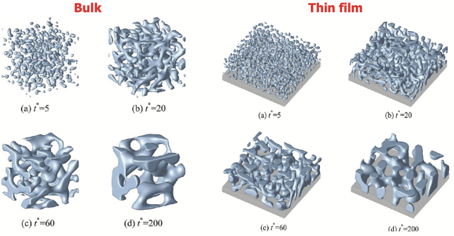
Example: spinodal decomposition in computer simulations
- See Seol, et al. Acta Materialia 51, 5173–5185 (2003)
- Final pattern always has a principal wavelength, why?
Interfacial energy as stabilization term
- The term \(R(\beta) = -\beta^2 \frac{M \Omega}{N_0} \frac{\partial^2 G}{\partial X_B^2}\) uses homogeneous free energy of a mixture
- In reality creating a new phase always increase the free energy by surface energy (similar to nucleation in Lecture 14)
- In spinodal decomposition, surface energy acts as “stablization” for pattern formation!
Energy at gradient interfaces
- Unlike in nucleation where sharp interface can be defined (thus \(\gamma\)), spinodal decomposition usually accompanies diffuse interface
- \(c_{B}\) has a finite gradient, not sharp step function
Additional term for interface gradient to Helmholtz free energy density
\[ f_{\gamma} = \kappa \left( \frac{\partial c_B}{\partial x} \right)^2 \]
- \(\kappa >0\) is the gradient energy coefficient that penalizes the creation of sharp interface
- At interface \(\left( \frac{\partial c_B}{\partial x} \right)^2\) becomes large!
Cahn-Hilliard equation for spinodal decomposition
- It is just Fick’s second law with a more precise \(\tilde{D}\) counting the interfacial term
- Total Helmholtz free energy comes from both homogeneous free energy density \(f^{\text{homo}}\) and \(\kappa (\partial c_B/\partial x)^2\)
Define a general “diffusion potential” for inhomogeneous system:
\[\begin{align} \Phi(x) &= \frac{\partial F}{V \partial cB} \\ &= \frac{\partial f^{\text{homo}}}{\partial c_B} - 2 \kappa \nabla^2 c_B \end{align}\]Cahn-Hilliard equation (2)
Instead of chemical potential \(\mu_B - \mu_A\), we use \(\Phi\) as the overall potential
- Fick’s 1st law
- Fick’s 2nd law
Cahn-Hilliard equation (3)
Final format of Cahn-Hilliard equation
\[\begin{align} \frac{\partial c_B}{\partial t} = M_0 \left[ \frac{\partial^2 f^{\text{homo}}}{\partial c_B^2} \nabla^2 c_B - 2 \kappa \nabla^4 c_B \right] \end{align}\]Perturbation analysis for Cahn-Hilliard equation
Toy model for the Helmholtz free energy
\[ f^{\text{homo}} = 16 \frac{f^{m}}{(c^\beta - c^\alpha)^4} \left[ (c_B - c^\alpha)(c_B - c^\beta) \right]^2 \]
How will the amplitude change?
\[ \frac{d A(t)}{dt} = \frac{M_0 \beta^2}{(c^\beta - c^\alpha)} \left[ 16 f^{m} - 2 \kappa \beta^2 (c^\beta - c^\alpha) \right] A(t) \]
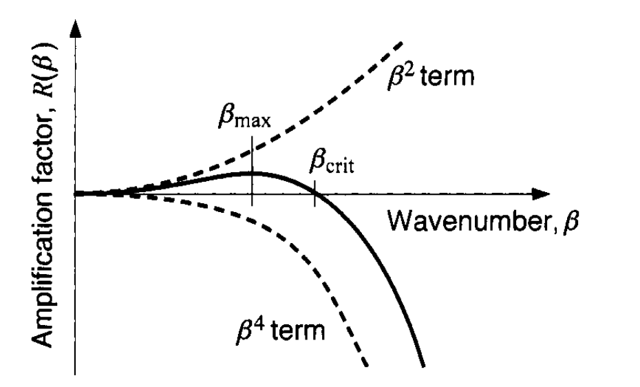
Amplification factor \(R(\beta)\) in Cahn-Hilliard equation
\[ R(\beta) = -M_0 \left( \frac{\partial^2 f}{\partial c_B^2} \beta^2 + 2 \kappa \beta^4 \right) \]
The \(\beta^4\) term now stablizes \(R(\beta)\)!
Cahn-Hilliard equation: critical wavelength
- Critical wavelength \(\lambda_c = \frac{\pi}{2} (c^\beta - c^\alpha) \sqrt{\frac{\kappa}{f^m}}\)
- \(\lambda > \lambda_c\) –> Growth
- Fastest growing wavelength \(\lambda_{\text{max}} = \sqrt{2} \lambda_c\)
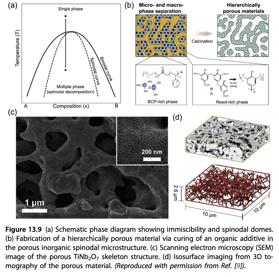
Applications of spinodal decomposition: pattern formation
Summary
- Continuous phase transformation is caused by initial composition inside the spinodal line (unstable region)
- Negative \(\tilde{D}\) causes spatial fluctuation to amplify
- Cahn-Hilliard equation describes the driving force
- Continuous phase separation occurs in many material systems and give rise to rich phase separation patterns