MATE 664 Lecture 20
Multiscale Simulation for Kinetics of Materials (I): Continuum Modelling
- Slides 👉 Open presentation🗒️
- PDF version of course note 👉 Open in pdf
- Handwritten notes 👉 Open in pdf
Learning outcomes
After this lecture, you will be able to:
- Recall the basic idea of continuum modelling in materials kinetics
- Identify the main ingredients of the Cahn-Hilliard and phase-field frameworks
- Describe how free energy, mobility, and gradient penalty enter a continuum model
- Interpret what phase-field simulations can predict for microstructure evolution
Why do we need material simulation?
- Modelling: how do we simplify the complex physical system?
- Simulation: how can the governing equation in a model evolve / be solved?
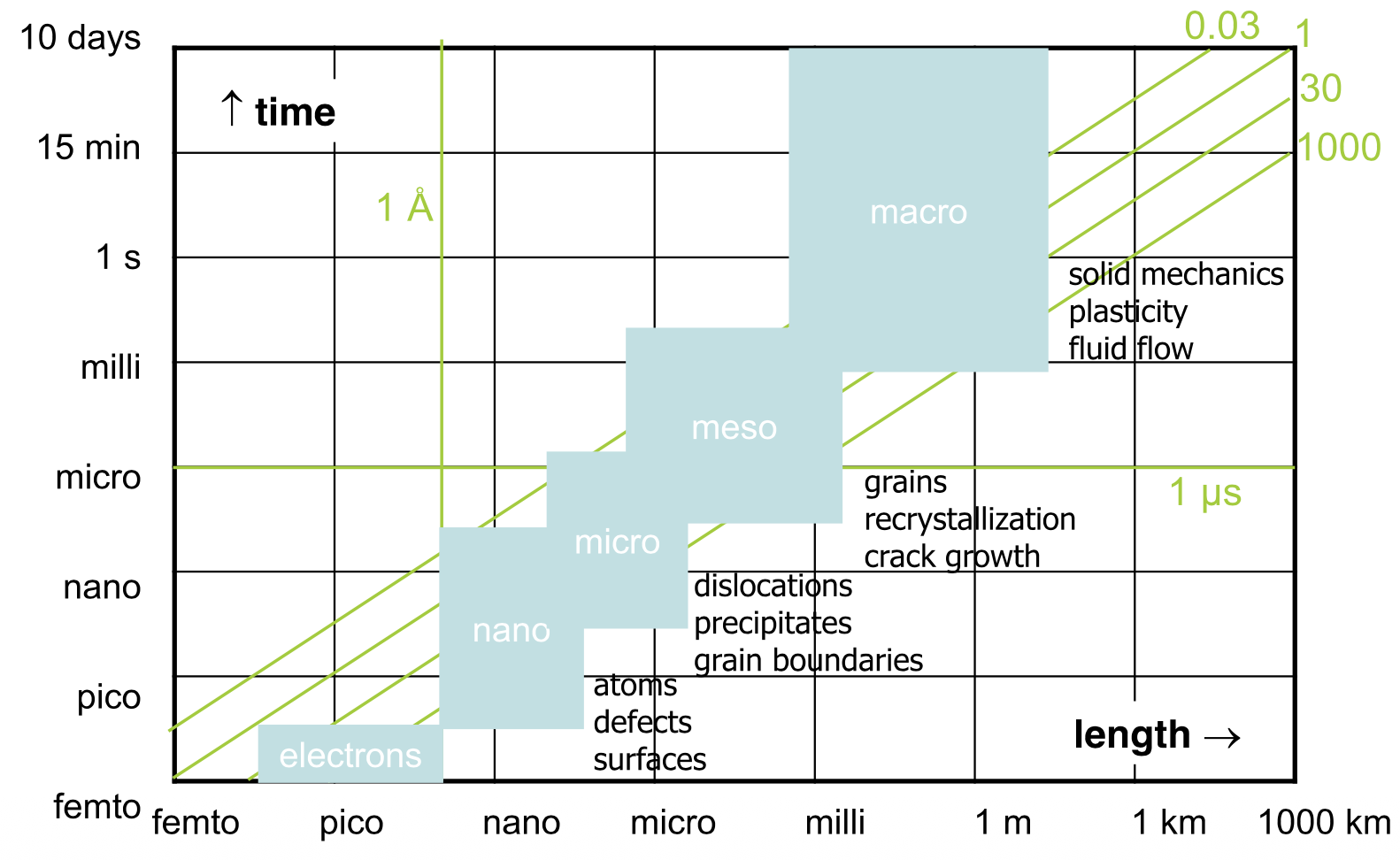
Multiscale modelling of materials
How do simulation methods differ at length scales?
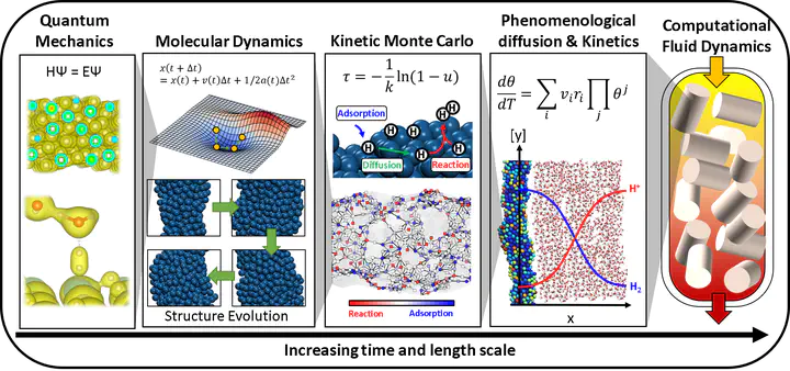
Multiscale view in spatial and temporal domains
Multiscale simulation in the context of kinetics

Topic 1: Continuum Modelling – Phase Field Method
What are we talking about in continuum modelling?
- Macroscopic diffusion – phenological diffusivity \(D\) is known
- Phase transformation – free energy of mixture system is known
Core equation: generalized Fick’s second law
\[ \frac{\partial \xi}{\partial t} = - \nabla \cdot \vec{J}_\xi(f, \xi) \]
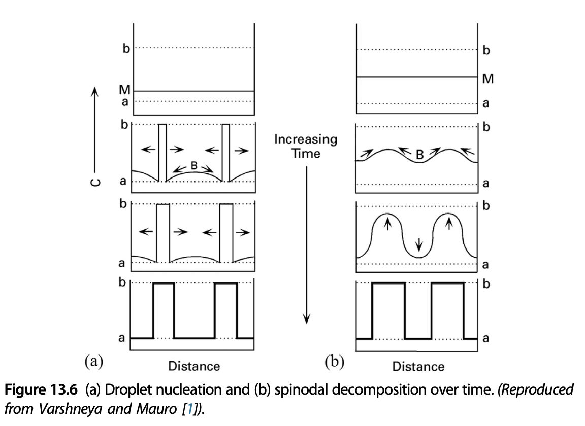
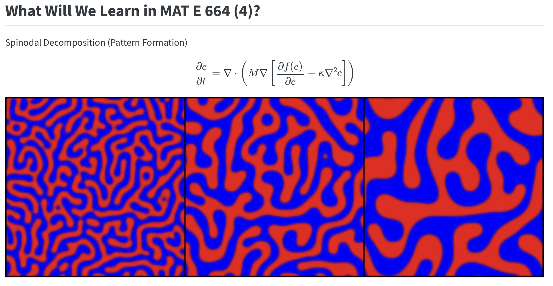
Case study: spinodal decomposition & nucleation
From Lecture 16 we know that the nucleation and spinodal decomposition of A-B mixture follows the same bulk free energy landscape while the time dependent evolution is different. How do we model it?
Target results
Review back to what we proposed in Lecture 1. Does this kind of image make sense?
Modelling step 1: check the governing equation
Problems suitable for continuum modelling typically have a clear governing equation, with a few parameters determined at bulk level or can be obtained from shorter-length scale simulations.
Can we identify the components for Cahn-Hilliard equation (L16)?
\[\begin{align} \frac{\partial c_B}{\partial t} = M_0 \left[ \frac{\partial^2 f^{\text{homo}}}{\partial c_B^2} \nabla^2 c_B - 2 \kappa \nabla^4 c_B \right] \end{align}\]CH equation analysis
\[\begin{align} \frac{\partial c_B}{\partial t} = M_0 \left[ \frac{\partial^2 f^{\text{homo}}}{\partial c_B^2} \nabla^2 c_B - 2 \kappa \nabla^4 c_B \right] \end{align}\]- \(f^{\text{homo}}\) is the homogeneous Helmholtz free energy
- \(M_0\) is the (non-negative) mobility under chemical potential driving force
- \(\kappa\): interfacial penalty
- Total concentration \(c_B\) and \(c_A\) should be conserved
Step 2: where do we get the free energy?
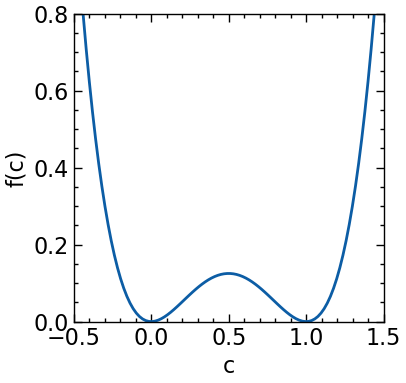
An easy choice of (homogeneous) Helmholtz free energy is the double well potential
\[\begin{align} f^{\text{homo}}(c_B) = W c_B^2 (1-c_B)^2 \end{align}\]- two minima: two preferred equilibrium compositions \(c_B=0\) and \(c_B=1\)
- barrier height set by \(W\)
Free energy and spinodal regions
Can you locate:
- Spinodal decomposition regime?
- Nucleation region?
From homogeneous to local free energy
In the Cahn-Hilliard equation the local free energy is defined
\[\begin{align} F(c_B) = \int_V \left[ f^{\text{homo}}(c_B) + \kappa |\nabla c_B|^2 \right] \mathrm{d}V \end{align}\]and subsequently we have a local chemical potential
\[\begin{align} \mu_B = \frac{\delta F}{\delta c_B} = \frac{\partial f^{\text{homo}}}{\partial c_B} - 2\kappa \nabla^2 c_B \end{align}\]The CH equation is just a diffusion equation with \(\nabla F(c_B)\) as the driving force.
What are the empirical parameters?
\[\begin{align} \frac{\partial c_B}{\partial t} = M_0 \left[ \frac{\partial^2 f^{\text{homo}}}{\partial c_B^2} \nabla^2 c_B - 2 \kappa \nabla^4 c_B \right] \end{align}\]For the simplest Cahn-Hilliard model, the key parameters are:
- \(W\): height of the double-well free energy barrier
- \(M_0\): mobility under chemical potential gradient
- \(\kappa\): gradient-energy coefficient
If the form of \(f^{\text{homo}}\) is fixed, this becomes a minimal 3-parameter model.
How do we set up the simulation?
The Cahn-Hilliard equation can be regarded as a showcase PDE problem in kinetics. In order to evolve the \(c_B\) field, we can use
Real space method:
- Finite different (FD): as in Lecture 8
- Finite element / finite volume: different ways to discretize the spatial grid
Fourier space method:
- Pseudo-spectral method: convert the real-space modes into Fourier space
Real space approach (high level)
A practical form is to split the equation into concentration and chemical potential:
\[\begin{align} \frac{\partial c_B}{\partial t} &= \nabla \cdot \left(M \nabla \mu_B \right) \\ \mu_B &= \frac{\partial f^{\text{homo}}}{\partial c_B} - 2\kappa \nabla^2 c_B \end{align}\]- the general form is just to solve the Fick’s second law with varying chemical potential space
- can use our existing FD code to update!
Fourier space strategy (high level)
Instead of solving the spatial derivatives directly in real space, we expand the concentration field into Fourier modes (the separation-of-variable method in Lecture 8). Note the notation \(c\) just means \(c_B\) in our previous case
\[\begin{align} c(\mathbf{r},t) = \sum_{\mathbf{k}} \hat{c}_{\mathbf{k}}(t)e^{i\mathbf{k}\cdot\mathbf{r}} \end{align}\]and the Fourier transform of the CH equation follows
\[\begin{align} \frac{\partial \hat{c}_{\mathbf{k}}}{\partial t} = M \left[ -k^2 \text{FT}[\frac{\partial f}{\partial c}] - \kappa k^4 \hat{c}_{\mathbf{k}} \right] \end{align}\]- \(\hat{c}_{\mathbf{k}}\) is the Fourier transformed \(c\)
- Benefit of F.T.: the \(\nabla^2\) and \(\nabla^4\) becomes just computing \(k^2\) and \(k^4\)
Example in action (1)
Adapted from PyCahnHilliard. Let’s see how the parameters change the result?
- At spinodal top
Example in action (2)
- More A phase
Example in action (3)
- More B phase
Evolution over time
Under the same free energy profile, how does the pattern evolve? And why?
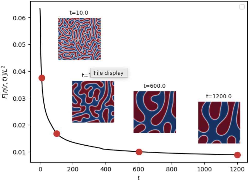
Interactive tool to play with the CH equation
Can you identify the following phenomena from the CH equation simulation?
- Nucleation
- Spinodal decomposition
- Coarsening
- Aggregation / sintering
Side note: CH equation interfacial thickness
The consequence of the CH equation is to have a diffuse interface, characterized by the width \(\lambda\):
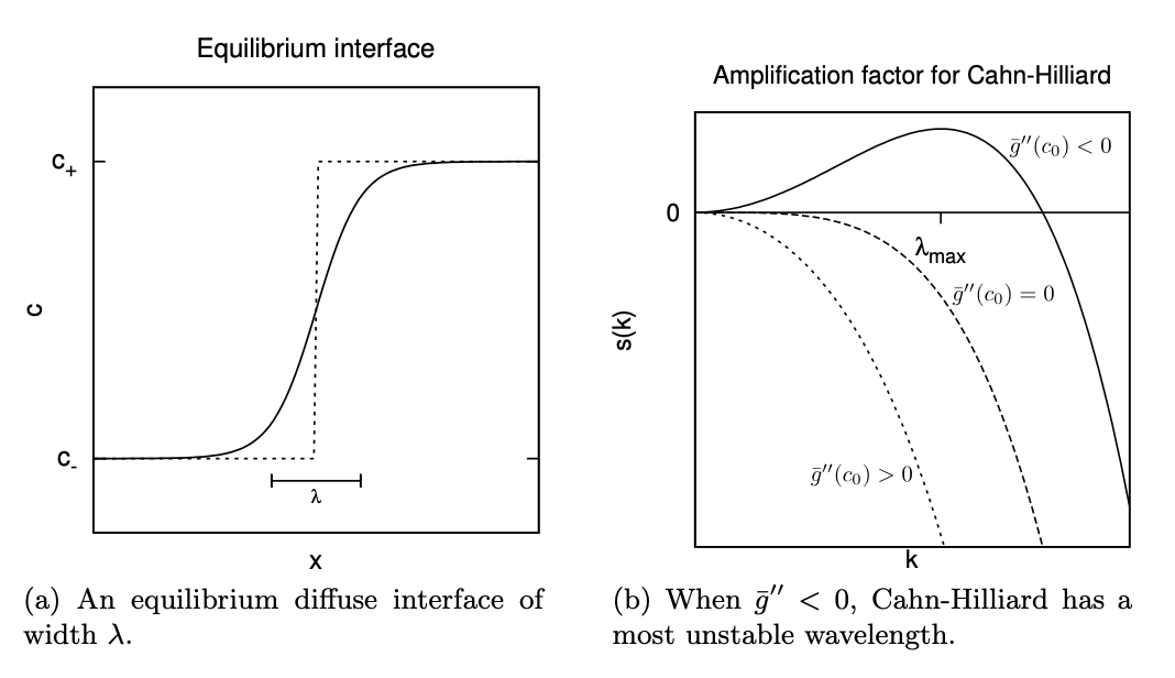
Side note: classical interfacial energy \(\gamma\) from CH picture
- The interfacial width \(\lambda\) is given by
\[ \lambda = \Delta c \sqrt{\frac{\kappa}{W}} \]
where \(W\) is the magnitude of the potential barrier
- The classical interfacial energy \(\gamma\) follows
What is the key message from Cahn-Hilliard?
- Thermodynamics enters through free energy \(f^{\text{homo}}\) (controlled by \(W\))
- Kinetics enters through mobility \(M\)
- Interface cost enters through gradient penalty (\(\kappa |\nabla c|^2\))
- Morphology evolves without explicitly setting interface
This is the core idea behind the phase field method.
From Cahn-Hilliard to phase field method
Cahn-Hilliard is one example of phase field modelling. General phase field strategy:
- choose a field variable \(\phi\) (the order parameter in Lecture 13)
- write a total free energy functional \(F(\phi, \cdots)\)
- obtain a driving force from variational derivative
- evolve the field with suitable dynamics
Why is phase field useful beyond this toy model?
- Moving interfaces do not need explicit tracking
- Morphology can be coupled to diffusion, stress, heat, or electrochemistry
- Suitable for realistic microstructure evolution problems
Example of solidification process in phase field modelling
See J. Braz. Soc. Mech. Sci. & Eng. 2011, 33, 125_.
- Heat transfer + phase transformation

What are the results?
Phase field simulation results yt video
Examples of phase field applications
- spinodal decomposition in alloys
- precipitate growth and coarsening
- dendritic solidification
- grain growth
- stress-coupled phase separation
- lithium concentration evolution in battery particles
Where to go next
The mathematical CH model does have a few parameters to be studied
- Free energy form?
- Free energy scale height?
- Molecular meaning of \(\kappa\)?
- Mobility \(M_0\)?
Not all continuum parameters can be predetermined –> get from simulations at other scales!
Summary
- Continuum modelling uses field variables and governing equations to describe kinetic evolution
- The Cahn-Hilliard equation combines bulk free energy, mobility, and interfacial penalty
- Phase-field methods extend this idea to simulate evolving microstructures without explicit interface tracking