MATE 664 Lecture 21
Multiscale Simulation (II): Monte-Carlo Methods
- Slides 👉 Open presentation🗒️
- PDF version of course note 👉 Open in pdf
- Handwritten notes 👉 Open in pdf
Learning outcomes
After this lecture, you will be able to:
- Recall the basic idea behind Monte Carlo methods in materials science
- Describe how Metropolis Monte Carlo samples equilibrium configurations
- Identify the main steps in a kinetic Monte Carlo algorithm
- Interpret when Monte Carlo methods are useful compared with continuum and molecular dynamics approaches
Recap: two ways for modelling large-scale motion in materials
- Continuum modelling / phase-field method: described by governing diffusion (Cahn-Hilliard type) equations
- Example: derivation of Einstein relation of diffusivity
- Discrete / event-based method: describe system as discrete steps
- Example: random walk model for diffusion
- Distinction:
- Do we have a continuum description of properties?
- Is probability easier to calculate?
Recap: comparison between scales

What is Monte Carlo method, anyway?
Monte Carlo (MC) methods describes a large set of stochastic methods to perform sampling in a (usually) high-dimensional space.
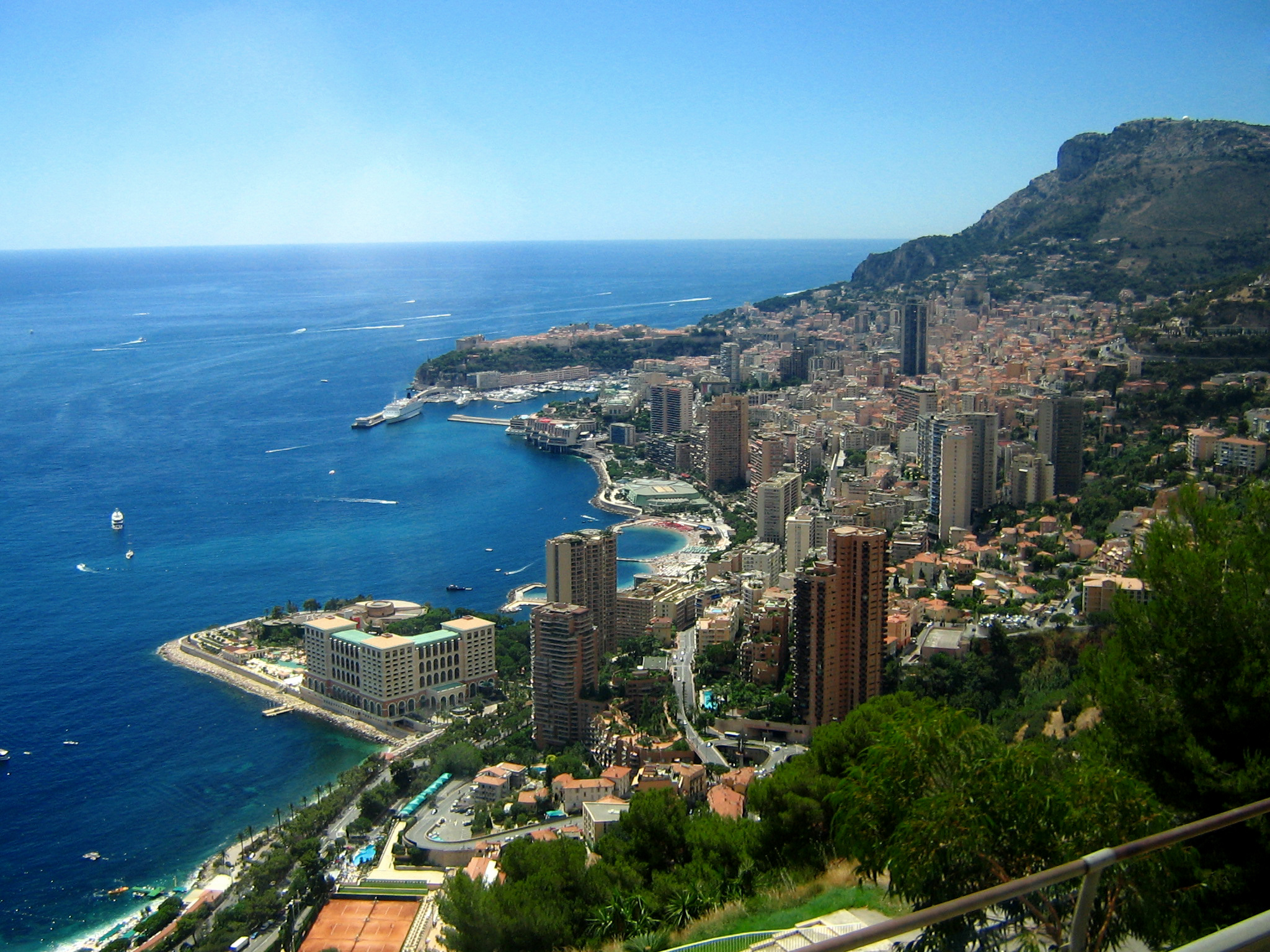
- Monte Carlo is part of the Principality of Monaco renowned for casino, luxurious hotels etc 👉 statistical mechanism was historically associated with gambling!
- First coined by von Neumann, Ulam, and Metropolis in Los Alamos to study neutron diffusion
- MC methods work surprisingly well for distribution in high-dimensional space, coupled with Bayesian statistics
Historical background for sampling-based method: Buffon’s needle problem
Buffon’s needle problem is one of the earliest demonstrations to estimate an unknown quantity (here \(\pi\)) via sampling. The probability of a needle with length \(l\) intersecting parallel lines spaced at \(d\) is:
\[ p = \frac{2}{\pi} \frac{l}{d} \]
- How does the estimation work?
- Recently proposed method for finding \(\pi\) using just coin-flip
Buffon’s needle problem: visualization
- How fast do the MC sampling converge?
- Can such integration be distributed over different systems?
Have we already seen a Monte Carlo simulation in our previous lectures?
Yes. The vacancy-mediated diffusion process (Lecture 9 & Assignment 2) shows this approach. We know that the macroscopic diffusion must follow the Fick’s equation
\[ J_A = -\tilde{D}\nabla c_A \]
and we can simulate the process (i.e. not knowing \(\tilde{D}\)) while only caring about the probabilities that a vacancy exchanges with a certain type of atom.
- Why are the probability picture and diffusion the same thing? 👉 See answers to Assignment 2
What do Monte Carlo simulations solve?
The following are taken from Landau and Binder, A Guide to Monte Carlo Simulations in Statistical Physics, (Cambridge U. Press, Cambridge U.K., 2000).
In a Monte Carlo simulation, we attempt to follow the ‘time dependence’ of a model for which change, or growth, does not proceed in some rigorously predefined fashion (e.g., according to Newton’s equations of motion) but rather in a stochastic manner which depends on a sequence of random numbers which is generated during the simulation.
Monte Carlo method vs molecular dynamics
The Monte Carlo (MD) method and Molecular Dynamics (MD) are both simulation techniques in material science but can be easily confused.
Similarity
- Use of potential energy / force field: the energy difference in MC and MD may be coming from similar or even the same potential energy equations
- Molecular representation: both MC and MD may be used to study exact atomic positions (explicit atom models) or coarse-grained models (groups of atoms)
- Ensemble: can be used in both cases
Difference
- MD simulations follow Newton’s equation
- (Usually) fixed time steps
- Calculation of forces (= gradient in energy) needed
- MC simulations use the probability between transitions
- Can advance in varied time steps (kinetic MC)
- Don’t need to calculate momenta / forces
Where does the probability come?
One main topic in the kinetics course is how to link the probability of a system to a certain energy scale. For a property \(A\) of interest, in the canonical (NVT) ensemble of system, such distribution follows the Boltzmann distribution
\[ \frac{p(A_i)}{p(A_j)} = \exp(- \frac{U_i - U_j}{k_B T}) \]
To estimate the expectation of \(A\) in NVT ensemble, we are required to calculate:
\[ \langle A \rangle_{NVT} = \frac{\int_\Omega A \exp(- \frac{U}{k_B T}) d\mathrm{r}} {\int_\Omega \exp(- \frac{U}{k_B T}) d\mathrm{r}} \]
How do we compute the integrals?
Mathematical form of Monte Carlo integration (I)
In the center of Monte Carlo methods, we are dealing with the integral of some (presummably) high-dimensional function \(f(\mathbf{x})\) on a domain \(\Omega=\{x_1, x_2, \cdots, x_n\}\), which can be transformed by another probability density function \(\rho(\mathbf{x})\)
\[\begin{align} F &= \int_{\Omega} f(\mathbf{x}) d \mathbf{x} \\ &= \int_{\Omega} \frac{f(\mathbf{x})}{\rho(\mathbf{x})} \rho(\mathbf{x}) d \mathbf{x} \end{align}\]and
\[ \rho(\mathbf{x}) \ge 0, \qquad \int_{\Omega} \rho(\mathbf{x})\, d\mathbf{x} = 1. \]
Mathematical form of Monte Carlo integration (II)
The integration problem for \(F\) now effectively becomes to find the expection for \(f / \rho\), when we draw samples \(x\) from the distribution \(\rho(x)\):
\[\begin{align} F &= \int_{\Omega} \frac{f(\mathbf{x})}{\rho(\mathbf{x})} \rho(\mathbf{x}) d \mathbf{x} \\ &= E\left[ \frac{f(\xi)}{\rho(\xi)} \right] \end{align}\]When the distribution \(\rho(x)\) is uniform, then we have
\[\begin{align} F \approx \frac{\Pi_{j=1}^{n} L_j }{N_{\text{trial}}} \sum_{i=1}^{N_{\text{trial}}} f(\xi_i) \end{align}\]where \(L_i\) is the domain size in dimension \(j\).
Mathematical form of Monte Carlo integration (III)
Why does the Monte Carlo method work? Compare the two ways to calculate \(F\)
- \(F\) by integration \(F = \int_{\Omega} f(\mathbf{x}) d \mathbf{x}\)
- Requires at least \(\text{npt}^n\) data points
- Intractable in high-dimensional space
- \(F\) by Monte Carlo sampling \(F \approx \frac{\Pi_{j=1}^{n} L_j }{N_{\text{trial}}} \sum_{i=1}^{N_{\text{trial}}} f(\xi_i)\)
- Requiring \({N_{\text{trial}}}\) sampling steps
- No exponential expansion with dimension (but may require convergence check)
- Performance differ by the choice of \(\rho\)
Statistical mechanics from MC perspective
The expectation value for \(A\) in a statistical mechanics system using a uniform sampling strategy is now:
\[ \langle A \rangle_{NVT} = \frac{\sum_i^{N_\text{trial}} A(\xi_i) \exp(- \frac{U(\xi_i)}{k_B T})} {\sum_{i}^{N_\text{trial}} \exp(- \frac{U(\xi_i)}{k_B T})} \]
This is a powerful conclusion! Every single thermodynamic quantity in the current ensemble can be estimated by random sampling. A long-enough MC simulation will eventually reveal the property.
Is this good enough? 
Problem with uniform-sampling Monte Carlo in materials simulations
The uniform-sampling MC method is not a feasible approach. There are a very large number of configurations that would be randomly generated that have effectively zero Boltzmann weight due to high-energy overlaps between the particles.
- Most points in the phase space: high-energy configurations 👉 extremely low probability
- Low energy configurations: physically observed states 👉 extremely low phase-space density
The solution: importance sampling / Metropolis-Hastings algorithm
The Metropolis-Hastings algorithm (I)
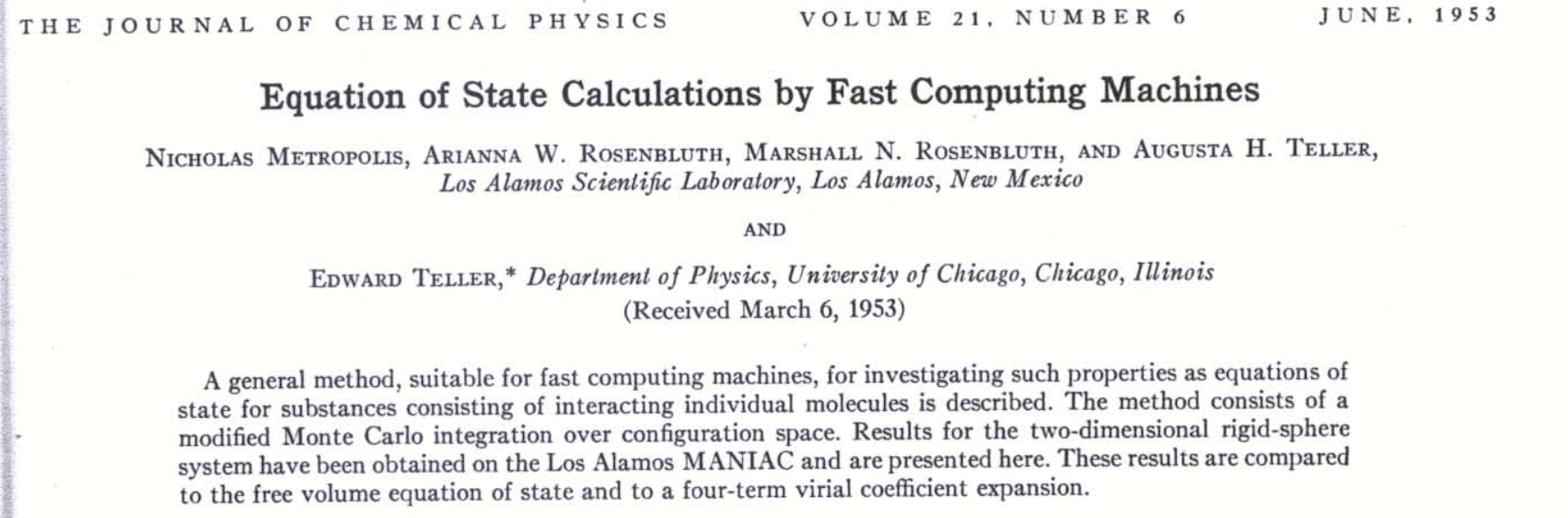
Originally proposed by Metropolis et al. in 1953 paper Equation of State Calculations by Fast Computing Machines. This is the basis of (almost) all MC sampling up to date:
The Metropolis-Hastings algorithm (II)
Let’s review the integral question again. Do we really need to use a uniform probability distribution \(\rho\), in systems that has Boltzmann behavious?
\[ F = \int_{\Omega} \frac{f(\mathbf{x})}{\rho(\mathbf{x})} \rho(\mathbf{x}) d \mathbf{x} \]
- Key idea: if \(\rho(\mathbf{x})\) is close to the actual \(f(\mathbf{x})\), the observed quantity during each sampling, \(\frac{f(\mathbf{x})}{\rho(\mathbf{x})}\) has little variance
- Problem: we don’t know what shape function \(f\) looks like, so can just guess.
- The best guess we could have is just the Boltzmann distribution
\[ \frac{p(A_i)}{p(A_j)} = \exp(- \frac{U_i - U_j}{k_B T}) \]
The Metropolis-Hastings algorithm (III)
Implementation of a Metropolis MC algorithm (in material science)
- Choose a random configuration
old\((x, y, z)\) coordinates of atoms - Generate a new configuration
newby either moving randoml distance or shift by lattice grids - Generate a uniq random number \(RN\)
- Calculate both potential energy \(U_{\text{old}}\) and \(U_{\text{new}}\)
- Accept the change if
\[ RN < \exp(-\frac{U_{\text{new}} - U_{\text{old}}}{k_B T}) \] 6. Goto step 2 and repeat
Metropolis MC: acceptance criteria
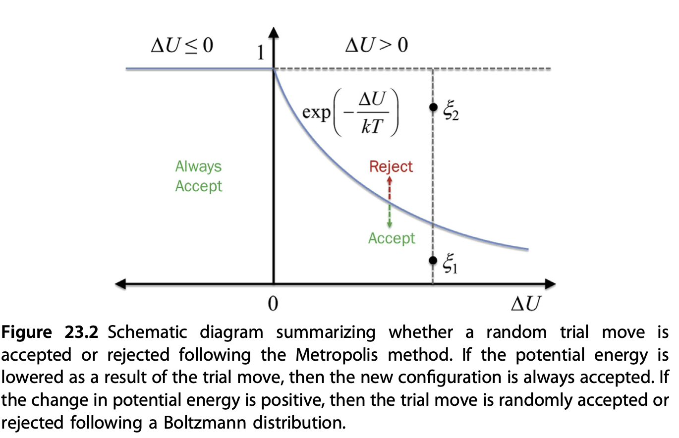
The Metropolis-Hastings algorithm: implications
- States with lower energy are always picked
- States with higher energy will be sampled up to a probability
The example belows shows the Metropolic MC 1D random walk. Observe its behaviour when inside the probability “peaks” (potential wells)
Metropolis MC: finding equilibrium state
The previous example shows that metropolis MC is able to find the equilibrium state of a system, even if we started away from that.
In contrast, standard molecular dynamics simulations are often hard to find other equilibria, if without proper biased sampling techniques
Have we seen something similar in the lecture notes before?
Metropolis MC demo: phase transformation simulation
Course materials from Lecture 12, Copyright: Vilas Winstein (UC Berkeley) Demo link. Youtube link
- Probability follow Boltzmann distribution \(p \propto \exp\left(-\frac{E + C N}{T}\right)\)
- Scaled potential / entropy \(C = T \mu = T \partial S/\partial N\)
- A modified grand canonincal Monte Carlo (GCMC) simulation: atoms can be inserted / removed to a reservoir with chemical potential \(C\)
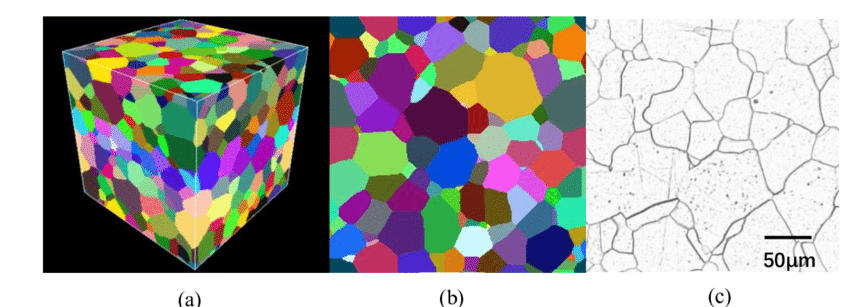
Metropolis MC: the Potts model for polycrystalline materials
Potts model (similar to the Icing model in solid-state physics) is a widely used technique to simulate the spatial composition domains in polycrystalline materials using the Monte Carlo method.
- Interested in:crystalline orientation \(q_i\) in each domain & how large the domains are
- Mathematical formulation:
\[ H = \sum_{\langle i,j\rangle} J \left(1 - \delta_{q_i,q_j}\right) \]
- \(\langle i,j\rangle\): neighboring lattice sites (up to 3rd- or 4-th neighbours)
- \(\delta_{q_i,q_j}=1\) if \(q_i=q_j\), otherwise \(0\): penalty for creating a grain boundary
- Different neighbors increase the energy \(\Rightarrow\) grain boundary energy
Potts model simulation
In a Metropolis MC simulation using the Potts model, Monte Carlo algorithm updates
- randomly choose a lattice site
- propose changing its state
- accept or reject using the Metropolis criterion
Monte Carlo in temporal domain: kinetic Monte Carlo (KMC)
From our previous examples we clearly see the (Metropolis) MC method is a powerful tool to reveal equilibrium composition, but what about systems that evolve over time?
Solution: Kinetic Monte Carlo (KMC)
- Provides much longer time scale than MD
- Probability comes from energy barrier / transition states
- Fundamentals from the Markov Chain (MC) process
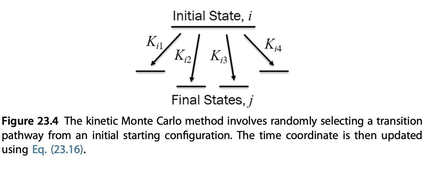
KMC in a nutshell
The KMC modelling is a special case of Markov-Chain Monte Carlo (MCMC), which tries to answer the question: how fast can I move from states to the other other.
- From each state \(i\), there are multiple states \(j\) that it can move to
- The rate of \(i \to j\) depends on the kinetic energy barrier between them
- From \(i \to j\), the most probable state is picked by considering all possible paths
- Time \(t\) is not explicitly used in the evolution but as a “process tracker”
KMC algorithm
We will introduce the direct method of KMC
Initialize the system at \(t=0\).
Find all possible transition paths for current state \(i\) either by:
- Eigenvector-following method
- Nudged-elastic band method
For each path, identify the end state \(k\)
Calculate individual rate \(k_{ij} = k_0 \exp(-\frac{E_{ij}^a}{k_B T})\) and total transition rates \(K = \sum_j k_{ij}\)
Pick a random number \(RN_1\), select the transition pathway \(i \to j_k\) that follows
\[ \sum_{j=1}^{j_k - 1} k_{ij} < RN_1 \cdot K < \sum_{j=1}^{j_k} k_{ij} \] 6. Move the system to state \(j_k\), and repeat step 2
Time handling in KMC simulation
If time needs to be tracked instead of the simulation steps, after selecting the pathway, the system time advances by
\[ \Delta t = -\frac{1}{K} \ln RN_2 \]
where \(RN_2\) is a second independent random number.
This is because for ANY of the first-order \(i \to j\) process to happen, the time scale is \(\frac{1}{K}\), while less likely events scales exponentially.
- First random number \(RN_1\): which process to happen?
- Second random number \(RN_2\): how long does it take to happen?
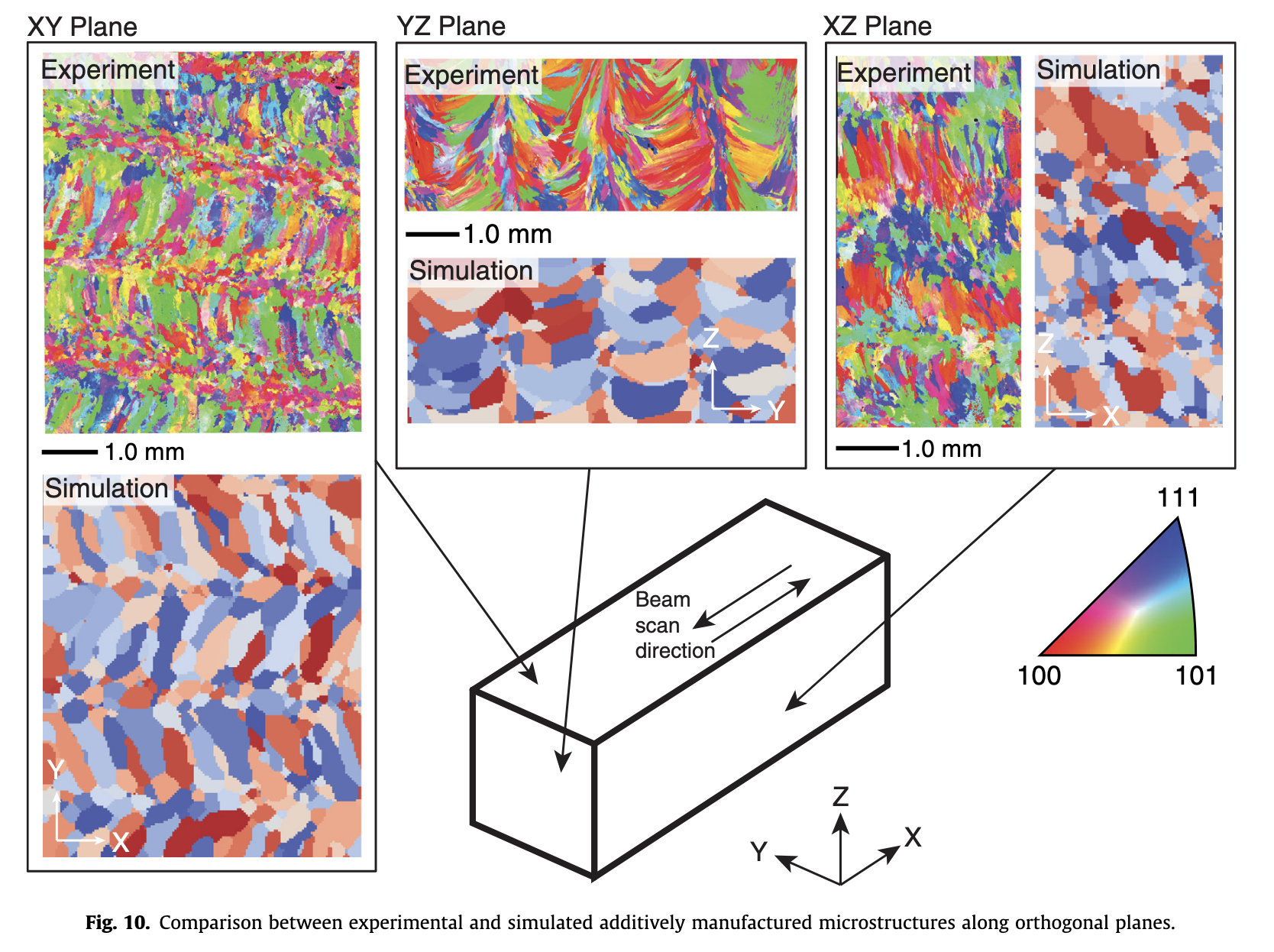
KMC simulation: additive manufacturing example
KMC simulation can handle much large length and timescales than MD.
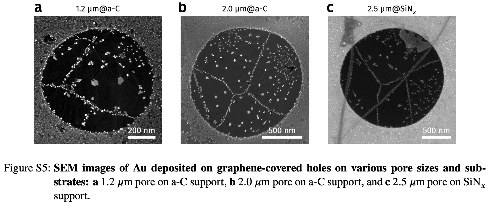
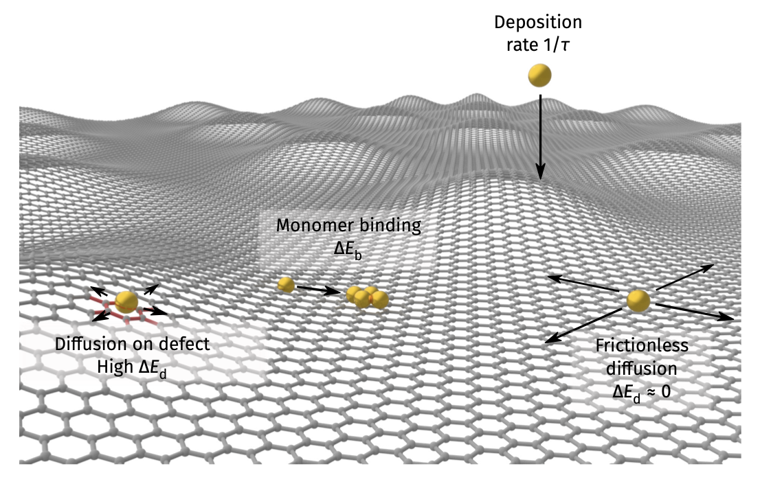
KMC example 2: deposition on graphene (previous Lecture 11)
- See Vagli and Tian et al. Nat Commun 2025, 16, 7726.
- Diffusivity change on free graphene surface can be probed by deposition geometry!
Deposition on Graphene - theoretical simulations
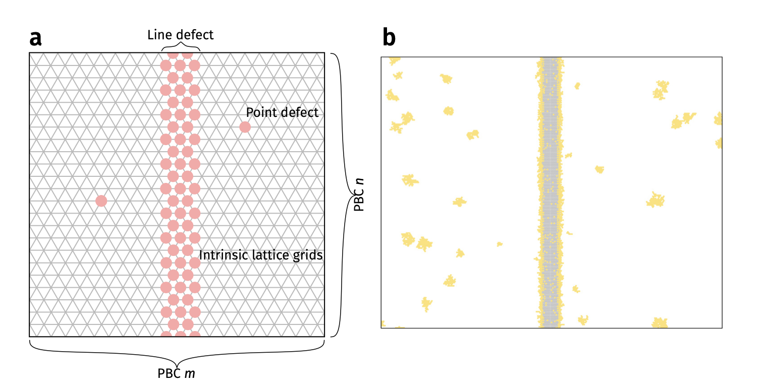
- Kinetic Monte Carlo (kMC) assuming different diffusion barrier on imperfections
- Faster diffusion direction –> lower density
Deposition on Graphene - theoretical simulations
- Kinetic Monte Carlo (kMC) assuming different diffusion barrier on imperfections
- Faster diffusion direction –> lower density
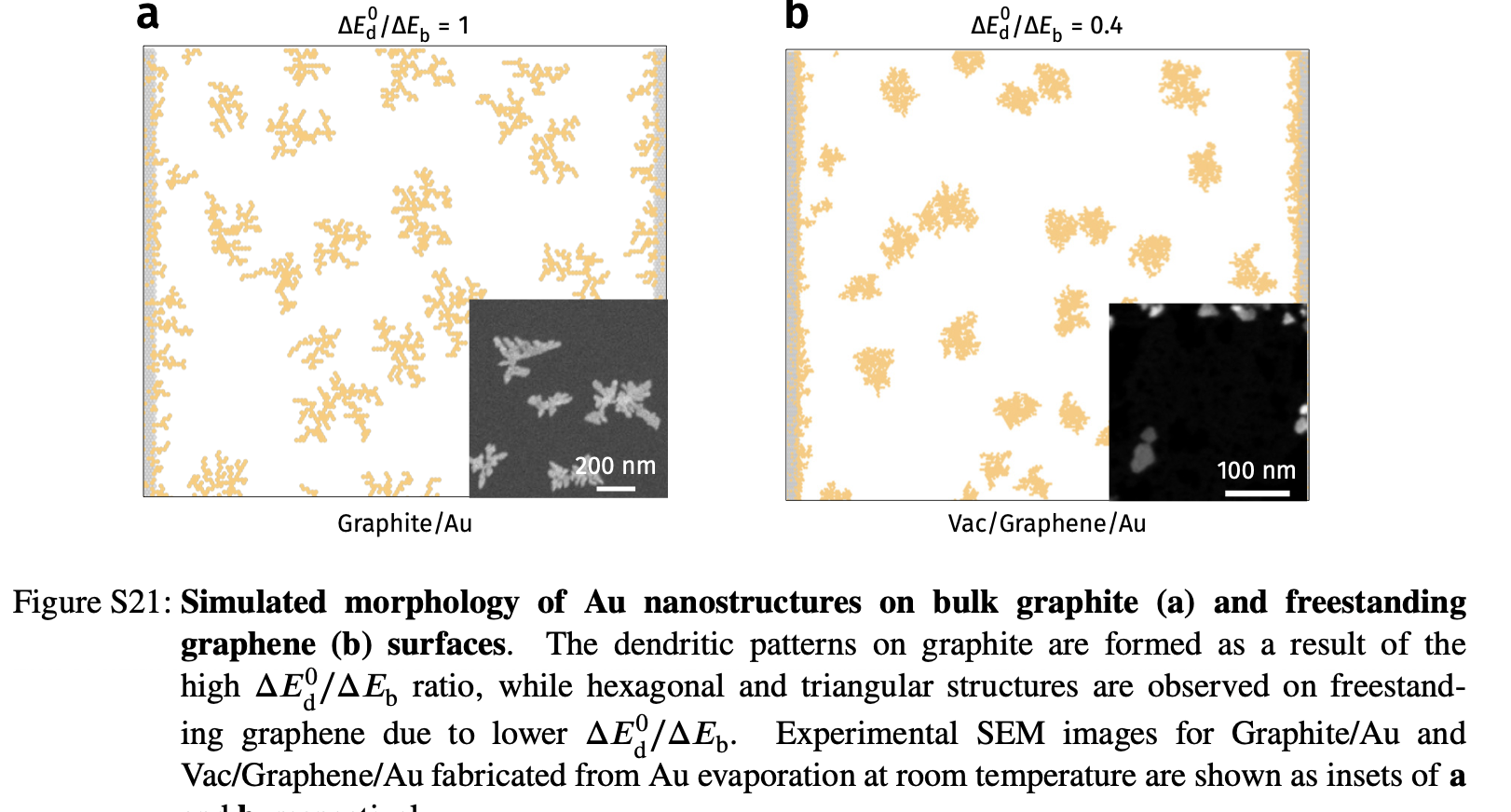
Deposition on Graphene - KMC vs experiments
Summary
- Monte Carlo methods use stochastic sampling to study materials problems that are difficult to solve deterministically
- Metropolis Monte Carlo targets equilibrium sampling, while kinetic Monte Carlo tracks rare events over time
- KMC links transition rates, pathway selection, and elapsed time in a discrete-event framework