CHE 318 Lecture 24
Mass Transfer In Two-Phase Column: Realistic Situations
- Slides 👉 Open presentation🗒️
- PDF version of course note 👉 Open in pdf
- Handwritten notes 👉 Open in pdf
Learning outcomes
After this lecture, you will be able to:
- Recall the stagnant-film flux relation for two-phase mass transfer.
- Apply film and equilibrium relations to determine interfacial compositions and fluxes.
- Describe how internal column mass balances shape local driving forces.
Recall of last week: two-phase mass transfer
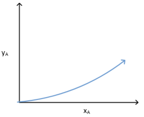
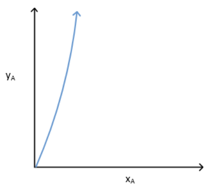
Useful tool: equilibrium diagram
Key features:
- x-axis & y-axis meaning?
- Points on and below curve?
- Equilibrium line and operating line?
- Points above and below eq. line?
- Meaning of operating line with flow rates?
![]()
Recap: key equation 1 – flux relation
For very diluted (EMCD-like) system, the flux equation in each phase follows:
\[\begin{align} N_A = k_y' (y_{AG} - y_{Ai}) = k_x' (x_{Ai} - x_{AL}) \end{align}\]This leads to the slope to the eq. line as:
\[\begin{align} \text{Slope} &= - \frac{y_{AG} - y_{Ai}}{x_{Ai} - x_{AL}} \\ &= -\frac{k_x'}{k_y'} \end{align}\]Recap: key equation 2 – mass balance (2-phase)
If we only care what possible \((x, y)\) points are in the tower, can use 2-phase mass balance:
\[\begin{align} L'\left(\frac{x_2}{1 - x_2}\right) + V'\left(\frac{y_1}{1 - y_1}\right) = L'\left(\frac{x_1}{1 - x_1}\right) + V'\left(\frac{y_2}{1 - y_2}\right) \end{align}\]In very diluted (EMCD-like) system, we have operating line with a slope of \(L'/V'\).
- Given inlet \(y_1\) and target \(x_2, y_2\) 👉 minimal operating \(L'\) (see Assignment 6!)
- Given actual \(L'\) 👉 predict outlet \(x_1\)
What can we improve from last week’s picture?
Applicability
- Instead of focusing on very diluted (\(1-x\approx 1-y \approx 1\)), derive equations for general, diffusion through stagnant film case
- Solving interfacial composition for general case
Case study: height requirement in packed absorption tower
- How tall should the tower / column be, given the mass transfer coefficients?
More accurate slope for interfacial connection
For non-dilute systems, \(1-x_{AL}\) and \(1-y_{AG}\) may not be close to
- The relation between \((x_{AL}, y_{AG})\) and \((x_{Ai}, y_{Ai})\) is no longer linear
- Need correction using log-mean composition terms
- Usual description: diffusion of \(A\) through non-diffusing \(B\)
Practical relation 1: flux relation for stagnant-film case
Still require the same flux through gas and liquid films:
\[\begin{align} N_A = \frac{k_y'}{(1-y)_{im}} (y_{AG}-y_{Ai}) = \frac{k_x'}{(1-x)_{im}} (x_{Ai}-x_{AL}) \end{align}\]So the line connecting bulk point to interface point has slope:
\[\begin{align} \text{Slope} &= \frac{y_{AG}-y_{Ai}}{x_{AL}-x_{Ai}} \\ &= -\frac{k_x'/(1-x)_{im}}{k_y'/(1-y)_{im}} \end{align}\]- uses: log mean correction \((1-x){im}\) and \((1-y){im}\)
- depend on the actual location
Note: log mean correction to interfacial flux
- The notations \((1 - x)_{im}\) and \((1 - y)_{im}\) are log mean values for inert composition between bulk and interface
- Just \(x_{Bm}\) in the steady-state diffusion problems
- Will be frequently used in this week’s lecture!
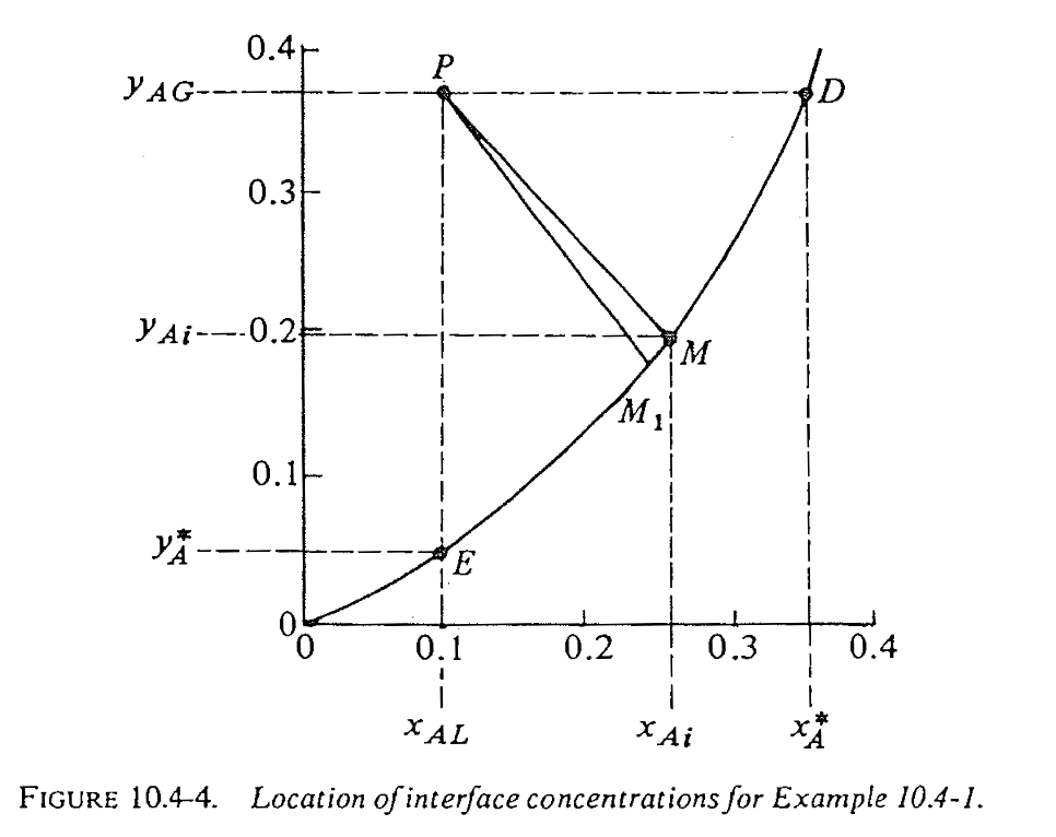
Example 1: finding the interfacial composition (stagnant B)
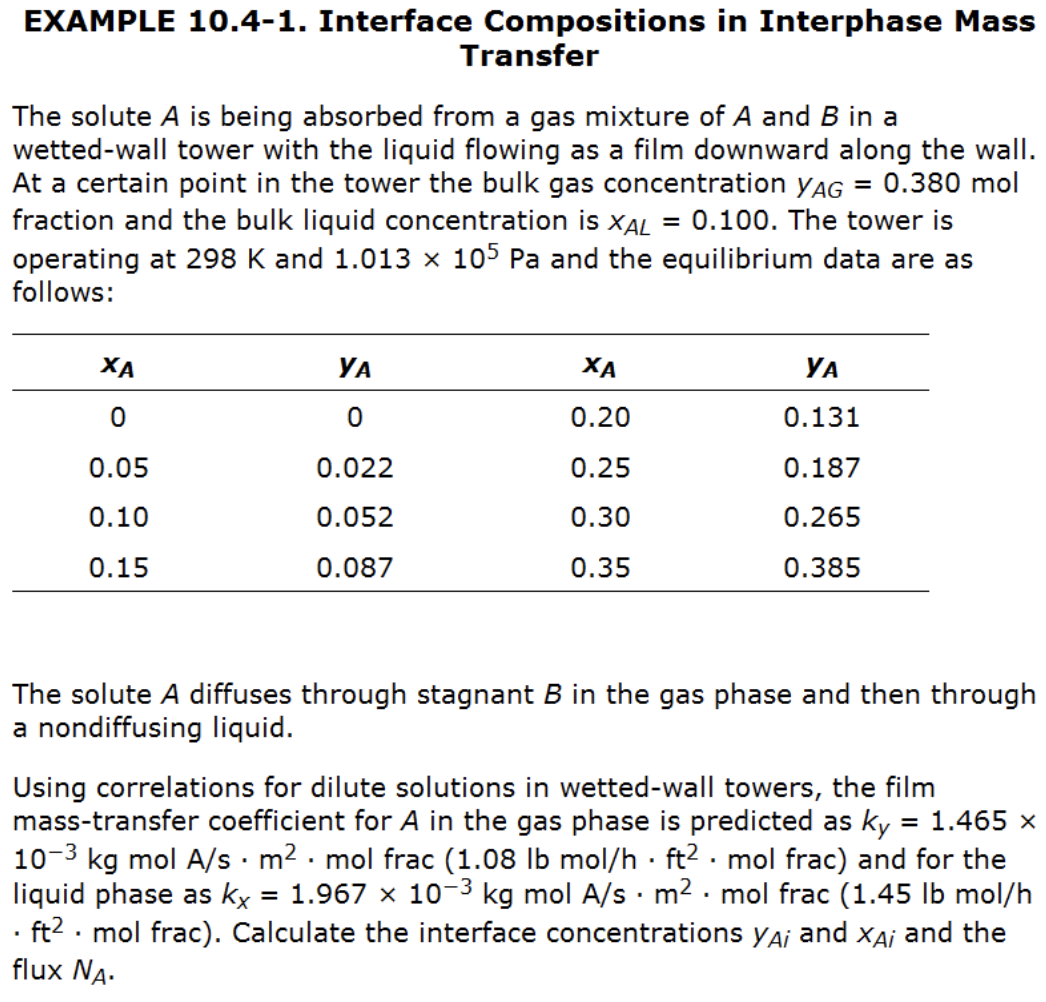
Solution steps for solving interfacial composition (general case)
Manual trial-and-error steps:
- Start from bulk point \(P\)
- Guess slope using current correction terms (initially \((1-x)_{im} = (1-y)_{im} = 1\))
- Connect to equilibrium curve to get \((x_{Ai}, y_{Ai})\)
- Update \((1-x){im}\) and \((1-y){im}\), calculate new slope
- Is new slope in 4) converged?
- No 👉 go back to step 2
- Yes 👉 continue to step 6
- Get final \((x_{Ai}, y_{Ai})\) and \(N_A\)
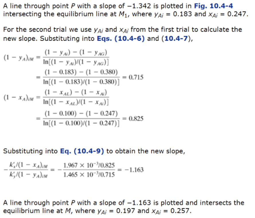
Example 1: step 1 (follow textbook)
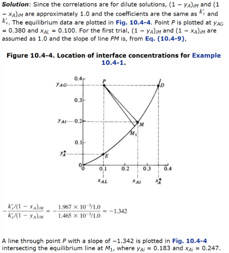
Example 1: step 2 (follow textbook)
Practical relation 2: link overall coefficient to film coefficients
- We learned last week that writing flux equations using \(K_x'\) and \(K_y'\) are usually easier than \(k_x'\) and \(k_y'\)
- What is the relation between them?
- Take gas-phase, diffusion through stagnant film
\((1-y)_{*m}\): log mean between \((1-y_{AG})\) and \((1-y_A^*)\)
Geometric interpretation of overall \(K\)
Use gas-phase example, from geometry of the equilibrium diagram:
\[\begin{align} \frac{1}{K_y}=\frac{1}{k_y}+\frac{m'}{k_x} \end{align}\]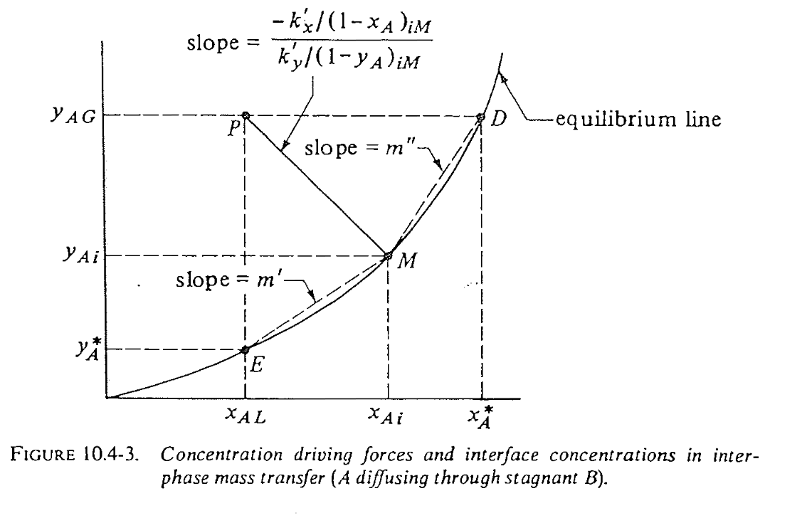
Transport resistance and overall mass transfer coefficients
- The overall mass transfer coefficient \(K\) basically tells which transport resistance is dominant (\(k\) inversely proportional to resistance)
- The transport equation becomes a “resistance-in-series” analog
Case 1: overall \(K_y\) in gas phase for highly liquid-soluble A
- Local slope \(m'\) is small
- Transfer resistance is mainly in gas!
- Design rule: tune \(k_y\) –> more efficient mass transfer
Case 2: overall \(K_x\) in liquid phase for low solubility A
- Local slope \(m''\) is large
- Transfer resistance is mainly in liquid!
- Design rule: tune \(k_x\) –> more efficient mass transfer
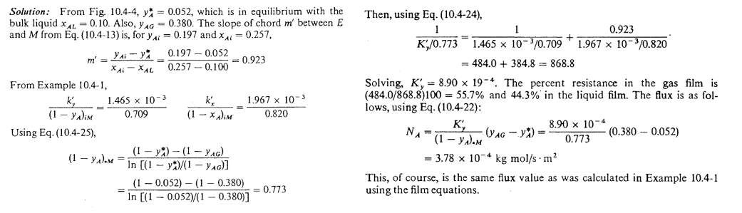
Example 2: estimate overall mass transfer coefficients
Use the conditions from example 1: bulk phase point \(P=(0.10, 0.380)\), \(k_x'=1.967\times 10^{-3}\) kg mol/m\(^2\)/s and \(k_y' = 1.465\times 10^{-3}\) kg mol/m\(^2\)/s, estimate \(K_y'\)?
Example 2: solutions
Summary
- In-depth analysis of diffusion through stagnant interfacial equilibrium
- Geometric interpretation of equilibrium diagram
- Case studies for interfacial composition & mass transfer coefficient
So far we have built almost all prerequisite for solving the concentration profile in the absorption tower! We will discuss that in upcoming Lecture 25