CHE 318 Lecture 25
Mass Transfer In Two-Phase Column: Concentration Profile
- Slides 👉 Open presentation🗒️
- PDF version of course note 👉 Open in pdf
- Handwritten notes 👉 Open in pdf
Learning outcomes
After this lecture, you will be able to:
- Recall the differential mass-balance framework for two-phase columns.
- Describe expressions for packed-column height from local transfer relations.
- Analyze coupled gas-liquid concentration profiles along the column.
Cheatsheet for packed bed design

Two-phase column: what have we learned so far?
For two-phase mass transfer (solid-state packed bed, liquid-gas absorption tower, etc.), our previous lectures have given:
What we have learned
- Equilibrium diagram ✅
- Operating line (dilute) ✅
- Overall mass balance ✅
- Interfacial composition ✅
What are still missing
- Concentration profile ❓
- Height requirement ❓
- Non-linear operating line ❓
In-depth analysis for packed absorption tower
Example goals:
- Analyze concentration profiles \(x(z)\) and \(y(z)\)
- Design packed-bed height \(z\)
Solution:
- Take a differential element of height \(dz\) 👉 differential equation
- Effective interfacial area: \(A_{\text{eff}} = aSdz\)
- Gas and liquid compositions both vary with \(z\)
Mass balance on control volume \(z \to z+dz\)
Mass balance for control volume still holds:
\[\begin{align} \text{In}_{liq} + \text{In}_{gas} = \text{Out}_{liq} + \text{Out}_{gas} \end{align}\]Governing equation for a slab with thickness \(dz\):
\[\begin{align} d(Vy)=d(Lx) \end{align}\]Flux equation in each phase
The relation \(d(Vy)=d(Lx)\) can be used to solve for each phase, if we know how to connect with flux equations individually.
Take the gas-phase side, the effective contact area being \(A_{\text{eff}}\) (see packed bed example in Lecture 21):
\[\begin{align} d(V y_{AG}) &= d(A_{\text{eff}}N_A) \\ &= \frac{k_y'}{(1-y_A)_{im}}(y_{AG}-y_{Ai})aSdz \end{align}\]note we need to account for the non-linear concentration profile by \(y_{Bm} = (1-y_A)_{im}\) as discussed in last lecture.
Governing differential equation for each phase
The part \(d(V y_{AG})\) can be further simplified, because we know \(V = V' / (1 - y_{AG})\):
\[\begin{align} d(Vy_{AG}) &= d(V'\frac{y_{AG}}{1-y_{AG}}) \\ &= V' \frac{1}{(1 - y_{AG})^2} d y_{AG} \end{align}\]The final differential form in gas phase is then:
\[\begin{align} V'\frac{1}{(1-y_{AG})^2}dy_{AG} = \frac{k_y'aS}{(1-y_A)_{im}}(y_{AG}-y_{Ai})dz \end{align}\]Differential equation for tower height
It is often desired to know the total height \(Z\) for the tower given operating line. We can integrate over the differential equation
\[\begin{align} Z &= \int_0^Z dz \\ &= \int_{y_2}^{y_1} \frac{V'}{k_y'aS} \cdot \frac{(1-y_A)_{im}}{(1-y_{AG})^2(y_{AG}-y_{Ai})} \, dy_{AG} \end{align}\]- this is the exact form for the gas-side height profile
- we can obtain the same equation using liquid-side conditions
- numerical integration is needed
Different forms of height equation
If we drop the subscript \(A\), and use \(V = V'/(1-y)\) & \(L=L'/(1-x)\), the height equation can be expressed in different forms
- Gas-side profile
\[ Z = \int_{y_2}^{y_1} \frac{V dy}{\frac{k'_y a S}{(1 - y)_{im}} (1 - y)(y - y_i)} \]
- Liquid-side profile
\[ Z = \int_{x_2}^{x_1} \frac{L dx}{\frac{k'_x a S}{(1 - x)_{im}} (1 - x)(x_i - x)} \]
The order of interface composition differences in liquid \((x_i - x)\) and gas \((y - y_i)\) have opposite signs!
Height equation using overall mass transfer coefficients
It is also possible to express the height equations using \(K_y'\) or \(K_x'\):
- Gas-side profile
\[ Z = \int_{y_2}^{y_1} \frac{V dy}{\frac{K'_y a S}{(1 - y)_{*m}} (1 - y)(y - y^*)} \]
- Liquid-side profile
\[ Z = \int_{x_2}^{x_1} \frac{L dy}{\frac{K'_x a S}{(1 - x)_{*m}} (1 - x)(x^* - x)} \]
The order of pseudo-interface composition differences in liquid \((x^* - x)\) and gas \((y - y^*)\) have opposite signs!
Simplified case: dilute system
The factors \(k_x'a\), \(k_y'a\), \(K_x'a\), \(K_y'a\) are usually not constant, making the solution harder to obtain. We will consider a simplified version of absorption of dilute gas.
- dilute regime: composition less than 0.1 (10 mol%)
- simplification 1: almost constant \(V\) and \(L\)
- simplification 2: \((1-x)_{im}/(1-x)\) and \((1-y)_{im}/(1-y)\) are almost independent on the location
- simplification 3: change of \(V\) (or \(L\)) over the column is minimal, usually use \(V = (V_1 + V_2)/2\)
Height equation in dilute systems
- Gas-side profile (use \(k'_y\))
\[ Z = \left[ \frac{V}{k'_y a S} \frac{(1 - y)_{im}}{1 - y} \right] \int_{y_2}^{y_1} \frac{dy}{y - y_i} \]
- Liquid-side profile (use \(k'_x\))
\[ Z = \left[ \frac{V}{k'_x a S} \frac{(1 - x)_{im}}{1 - x} \right] \int_{x_2}^{x_1} \frac{dx}{x_i - x} \]
Replacing \(_{im}\) subscripts with \(_{*m}\) and using overall coefficients gives another set of equations.
Further simplification: log mean driving force
In practical cases we can even let \(\frac{(1 - y)_{im}}{1 - y} \approx 1\) and \(\frac{(1 - x)_{im}}{1 - x} \approx 1\). The R.H.S. becomes only dependent on \(\int_{y_2}^{y_1} \frac{dy}{y - y_i}\).
\[\begin{align} Z &= \frac{V}{k_y'aS} \int_{y_2}^{y_1} \frac{dy}{y - y_i} \frac{V}{k_y'aS} \ln\left(\frac{y_1-y_i}{y_2-y_i}\right) \end{align}\]From the packed-bed analysis in Lecture 21 we know it corresponding to a log-mean driving force term \((y - y_i)_{m}\):
\[\begin{align} \frac{V}{S}(y_1-y_2) &= k_y'aZ \frac{(y_1-y_i)-(y_2-y_i)} {\ln\left(\dfrac{y_1-y_i}{y_2-y_i}\right)} \\ &= k_y' aZ (y - y_i)_{m} \end{align}\]What does the result tell us?
Let’s take a pause and check the meaning for the governing equation
\[\begin{align} \frac{V}{S}(y_1-y_2) = k_y' aZ (y - y_i)_{m} \end{align}\]- L.H.S.: molar flow of A absorbed per column cross-sectional area
- R.H.S.: molar flow of A transferred from gas to liquid phase
- average driving force: log-mean of \(y-y_i\)
- transfer coefficient: \(k_y'\)
Visualization of log-mean driving force
For dilute gas system, the driving force can be visualized using diagonal lines connecting the operating line and equilibrium line.

Comparison: packed bed with solid spheres
The dilute two-phase system is very close to the packed bed of solid spheres in Lecture 21, see the side-by-side comparison.
Packed bed of solid spheres
- Constant \(c_{Ai}\)
- Uses log-mean driving force of \(c\)
\[ Q(c_2 - c_1) = k_c' a H (c_i - c)_{m} \]
Packed bed of liquid-gas
- Varying \(y_i\)
- Uses log-mean driving force of \(y\)
\[ \frac{V}{S}(y_1 - y_2) = k_y' a Z (y - y_i)_{m} \]
All forms of height equation in dilute system
- Gas, use \(k_y'\)
\[ \frac{V}{S}(y_1 - y_2) = k_y' a Z (y - y_i)_{m} \]
Liquid, use \(k_x'\) \[ \frac{V}{S}(x_1 - x_2) = k_x' a Z (x_i - x)_{m} \]
Gas, use \(K_y'\)
\[ \frac{V}{S}(y_1 - y_2) = K_y' a Z (y - y^*)_{m} \]
- Liquid, use \(K_x'\) \[ \frac{V}{S}(x_1 - x_2) = K_x' a Z (x^* - x)_{m} \]
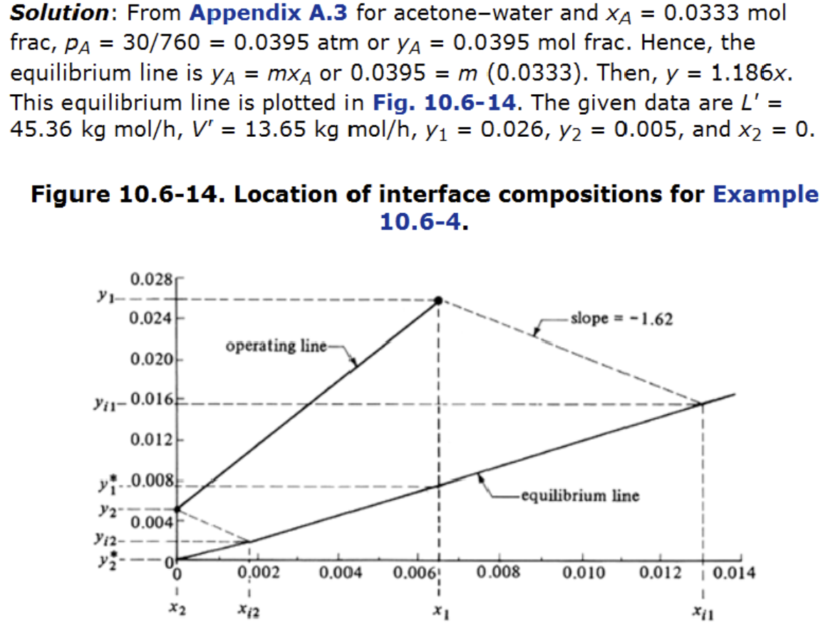
Example: calculate height of acetone absorption tower
(Example 10.6-4) Acetone is being absorbed by water in a packed bed column having a cross sectional area of 0.186 m\(^2\) at 293 K and 1 atm. The inlet air contains 2.6 mol% acetone and outlet contains 0.5%. The gas flow is 13.65 kg mol inert air per hour. The pure water inlet flow is 45.36 kg mol water per hour. The coefficient \(k_y' a\) is estimated to be \(3.78 \times 10^{-2}\) kg mol/(s·m\(^3\)) and \(k_x' a\) is \(6.16 \times 10^{-2}\) kg mol/(s·m\(^3\)). The equilibrium line can be approximated by
\[ y = 1.186 x \]
- calculate the tower height use \(k_y' a\)
- repeat a) but use \(k_x' a\)
- calculate the tower height use \(K_y' a\)
Solution steps (1)
Is this system dilute (<10%)?
Yes. Choose linear operating line and height equation
Determine two ends of the operating line
- Point 1: \(x_1\)=?; \(y_1=0.026\)
- Point 2: \(x_2=0\); \(y_2=0.005\)
- Calculate \(x_1\)?
Use mass balance equation
Solution steps (2)
- Find the slope of curve
Solutions steps (3)
- To use the height equation
\[ \frac{V}{S}(y_1 - y_2) = k_y' a Z (y - y_i)_{m} \]
- total flow rate \(V=\frac{V_1 + V_2}{2}\approx 3.852 \times{} 10^{-3}\) kg mol/s
- log-mean driving force
\[ (y - y_i)_{m} = \frac{(y_1 - y_i) - (y_2 - y_i)}{\ln (\frac{y_1 - y_i}{y_2 - y_i})} = 0.006 \]
Final result: \(Z=1.911\) m
Summary
- Solving single-phase mass balance in absorption packed tower
- Use dilute solution for tower height analysis
- Recall the analog between the solid sphere packed bed and liquid-gas tower
\[ (1 - y)_{im} = \frac{(1 - y_{AG}) - (1 - y_{Ai})}{\ln\! \frac{1 - y_{AG}}{1 - y_{Ai}}} \]
\[ (y - y_i)_{m} = \frac{(y_{1} - y_{i1}) - (y_{2} - y_{i2})}{\ln\! \frac{y_{1} - y_{i1}}{y_2 - y_{i2}}} \]